How to Create an Image Histogram Using OpenCV

Given an image as input, how do we get the corresponding histogram using OpenCV? First, let us take a look at what a histogram is, then let us take a look at how to create one given an image.

What is a Histogram?

A histogram is another way of looking at an image. It is a graph that shows pixel brightness values on the x-axis (e.g. 0 [black] to 255 [white] for grayscale images) and the corresponding number (i.e. frequency) of pixels (for each brightness value) on the y-axis.

How to Create an Image Histogram Using OpenCV

There are two links I particularly like that show how to create the image histogram given an input image.

I like these tutorials because they lead the reader through all the essentials of how to find and analyze image histograms, step-by-step. This process boils down to the following code:

# Import the required libraries
import cv2  # Open CV
from matplotlib import pyplot as plt  #Matplotlib for plotting  
 
# Read the input image
img = cv2.imread('example.jpg',0) 
 
# Calculate the frequency of pixels in the brightness range 0 - 255
histr = cv2.calcHist([img],[0],None,[256],[0,256]) 
 
# Plot the histogram and display
plt.plot(histr) 
plt.show()

Why Use CMOS Instead of CCD Sensors in Mobile Phones

If I were designing a new state-of-the-art mobile phone, I would choose Complementary metal–oxide–semiconductor (CMOS). CMOS has several advantages over a Charge-coupled device (CCD), which I will explain below.

Processing Speed

In CCD, photosites are passive, whereas in CMOS they are not…leading to slower processing speed and information transfer.

A photosite is denoted as a single color pixel in a CCD or CMOS sensor. In a CCD sensor, light is captured and converted into a charge. The charge accumulates in the photosites, is transferred to a voltage converter, and is then amplified. This whole process happens one row at a time. This video below demonstrates this process.

However, with a CMOS sensor, the charge to voltage conversion and the amplification of the voltage occurs inside each photosite. Because the work on an image happens locally, processing and information transfer is faster than a CCD sensor.

Space Requirements

CMOS enables integration of timers and analog-to-digital converters, which conserves space.

CCD is an older technology, and it is not possible to integrate peripheral components like analog-to-digital converters and timers on a single chip. CMOS does enable integration of these components onto a single chip, which conserves space.

For a mobile phone that needs to be limited to a certain size, space must be conserved, which gives CMOS an advantage for use in mobile phones.

Power Consumption

CCD consumes more power than CMOS. CCD needs a variety of power supplies for the timing clocks. Also, it requires a voltage of 7V to 10V.

A CMOS sensor requires just one power supply and requires a voltage of 3.3V to 5V, roughly 50% less than a CCD sensor. This lower power consumption means extended battery life.

CMOS Prevents Blooming

In a CCD sensor, when an image is overexposed, electrons pile up in the areas of the brightest part of the image and overflow to other photosites, which creates unwanted light streaks. The structure of CMOS sensors prevents this problem.

Cost

CMOS chips can be produced on virtually any standard silicon production line, whereas this is not the case for CCD chips. As a result, production cost is lower for CMOS chips. These cost savings result in better profit margins for mobile phone companies.

How to Draw the Letter ‘E’ on an Image Using Scikit-Image

Requirements

Develop a program in Python to draw an E at the center of an input image.

Program must be developed using Python 3.x.
Program must use scikit-image library — a simple and popular open source library for image processing in Python.
The input image must be a color image.
The letter must be at the center of the image and must be created by updating pixels, not by using any of the drawing functions.
The final output must be a side-by-side image created using matplotlib.
Must test the same code with two different images or two different sizes.

You Will Need

Anaconda and Jupyter Notebooks or a Python IDE

Directions

Find any two images/photos.

Create a new Jupyter Notebook.

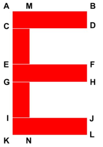
Here are the critical reference points for the letter E. These points mark the corners of the four rectangles that make up the letter E.

Here is the pdf of my Jupyter notebook.

Here is the raw code for the program in Python:

#!/usr/bin/env python
# coding: utf-8

# # Project 1 – Introduction to Python scikit-image
# 
# ## Author
# Addison Sears-Collins
# ## Date Created
# 9/4/2019
# ## Python Version
# 3.7
# ## Description
# This program draws an E at the center of an input image.
# ## Purpose
# The purpose of this assignment is to introduce the basic functions of the Python scikit-image
# library -- a simple and popular open source library for image processing in Python. The scikitimage
# extends scipy.ndimage to provide a set of image processing routines including I/O, color
# and geometric transformations, segmentation, and other basic features.
# ## File Path

# In[1]:


# Move to the directory where the input images are located
get_ipython().run_line_magic('cd', 'D:\\Dropbox\\work')

# List the files in that directory
get_ipython().run_line_magic('ls', '')


# ## Code

# In[2]:


# Import scikit-image
import skimage

# Import module to read and write images in various formats
from skimage import io

# Import matplotlib functionality
import matplotlib.pyplot as plt

# Import numpy
import numpy as np

# Set the color of the E
# [red, green, blue]
COLOR_OF_E = [255, 0, 0]


# In[3]:


# Show the critical points of E
from IPython.display import Image
Image(filename = "e_critical_points.PNG", width = 200, height = 200)


# In[4]:


def e_generator(y_dim, x_dim):
    """
    Generates the coordinates of the E
    :param y_dim int: The y dimensions of the input image
    :param x_dim int: The x dimensions of the input image
    :return: The critical coordinates
    :rtype: list
    """
    # Set all the critical points
    A =  [int(0.407 * y_dim), int(0.423 *  x_dim)]
    B =  [int(0.407 * y_dim), int(0.589 *  x_dim)]
    C =  [int(0.488 * y_dim), int(0.423 *  x_dim)]
    D =  [int(0.488 * y_dim), int(0.589 *  x_dim)]
    E =  [int(0.572 * y_dim), int(0.423 *  x_dim)]
    F =  [int(0.572 * y_dim), int(0.581 *  x_dim)]
    G =  [int(0.657 * y_dim), int(0.423 *  x_dim)]
    H =  [int(0.657 * y_dim), int(0.581 *  x_dim)]
    I =  [int(0.735 * y_dim), int(0.423 *  x_dim)]
    J =  [int(0.735 * y_dim), int(0.589 *  x_dim)]
    K =  [int(0.819 * y_dim), int(0.423 *  x_dim)]
    L =  [int(0.819 * y_dim), int(0.589 *  x_dim)]
    M =  [int(0.407 * y_dim), int(0.47 *  x_dim)]
    N =  [int(0.819 * y_dim), int(0.47 *  x_dim)]
    
    return A,B,C,D,E,F,G,H,I,J,K,L,M,N


# In[5]:


def plot_image_with_e(image, A, B, C, D, E, F, G, H, I, J, K, L, M, N):
    """
    Plots an E on an input image
    :param image: The input image
    :param A, B, etc. list: The coordinates of the critical points
    :return: image_with_e
    :rtype: image
    """
    # Copy the image
    image_with_e = np.copy(image)

    # Top horizontal rectangle
    image_with_e[A[0]:C[0], A[1]:B[1], :] = COLOR_OF_E 

    # Middle horizontal rectangle
    image_with_e[E[0]:G[0], E[1]:F[1], :] = COLOR_OF_E

    # Bottom horizontal rectangle
    image_with_e[I[0]:K[0], I[1]:J[1], :] = COLOR_OF_E

    # Vertical connector rectangle
    image_with_e[A[0]:K[0], A[1]:M[1], :] = COLOR_OF_E

    # Display image
    plt.imshow(image_with_e);

    return image_with_e


# In[6]:


def print_image_details(image):
    """
    Prints the details of an input image
    :param image: The input image
    """
    print("Size: ", image.size)
    print("Shape: ", image.shape)
    print("Type: ", image.dtype)
    print("Max: ", image.max())
    print("Min: ", image.min())


# In[7]:


def compare(original_image, annotated_image):
    """
    Compare two images side-by-side
    :param original_image: The original input image
    :param annotated_image: The annotated-version of the original input image
    """
    # Compare the two images side-by-side
    f, (ax0, ax1) = plt.subplots(1, 2, figsize=(20,10))

    ax0.imshow(original_image)
    ax0.set_title('Original', fontsize = 18)
    ax0.axis('off')

    ax1.imshow(annotated_image)
    ax1.set_title('Annotated', fontsize = 18)
    ax1.axis('off')


# In[8]:


# Load the test image
image = io.imread("test_image.jpg")

# Store the y and x dimensions of the input image
y_dimensions = image.shape[0]
x_dimensions = image.shape[1]

# Print the image details
print_image_details(image)

# Display the image
plt.imshow(image);


# In[9]:


# Set all the critical points of the image
A,B,C,D,E,F,G,H,I,J,K,L,M,N = e_generator(y_dimensions, x_dimensions)

# Plot the image with E and store it
image_with_e = plot_image_with_e(image, A, B, C, D, E, F, G, H, I, J, K, L, M, N)

# Save the output image
plt.imsave('test_image_annotated.jpg', image_with_e)


# In[10]:


compare(image, image_with_e)


# In[11]:


# Load the first image
image = io.imread("architecture_roof_buildings_baked.jpg")

# Store the y and x dimensions of the input image
y_dimensions = image.shape[0]
x_dimensions = image.shape[1]

# Print the image details
print_image_details(image)

# Display the image
plt.imshow(image);


# In[12]:


# Set all the critical points of the image
A,B,C,D,E,F,G,H,I,J,K,L,M,N = e_generator(y_dimensions, x_dimensions)

# Plot the image with E and store it
image_with_e = plot_image_with_e(image, A, B, C, D, E, F, G, H, I, J, K, L, M, N)

# Save the output image
plt.imsave('architecture_roof_buildings_baked_annotated.jpg', image_with_e)


# In[13]:


compare(image, image_with_e)


# In[14]:


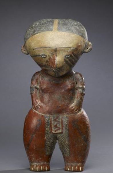
# Load the second image
image = io.imread("statue.jpg")

# Store the y and x dimensions of the input image
y_dimensions = image.shape[0]
x_dimensions = image.shape[1]

# Print the image details
print_image_details(image)

# Display the image
plt.imshow(image);


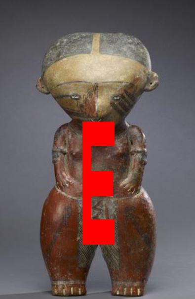
# In[15]:


# Set all the critical points of the image
A,B,C,D,E,F,G,H,I,J,K,L,M,N = e_generator(y_dimensions, x_dimensions)

# Plot the image with E and store it
image_with_e = plot_image_with_e(image, A, B, C, D, E, F, G, H, I, J, K, L, M, N)

# Save the output image
plt.imsave('statue_annotated.jpg', image_with_e)


# In[16]:


compare(image, image_with_e)


# In[ ]:

Tag: image processing

How to Create an Image Histogram Using OpenCV

What is a Histogram?

How to Create an Image Histogram Using OpenCV

Why Use CMOS Instead of CCD Sensors in Mobile Phones

Processing Speed

Space Requirements

Power Consumption

CMOS Prevents Blooming

Cost

How to Draw the Letter ‘E’ on an Image Using Scikit-Image

Requirements

You Will Need

Directions

Example

Before

After