In this post, I will walk you through the Logistic Regression algorithm step-by-step.
- We will develop the code for the algorithm from scratch using Python.
- We will run the algorithm on real-world data sets from the UCI Machine Learning Repository.
Table of Contents
- What is Logistic Regression?
- Logistic Regression Algorithm Design
- Logistic Regression Algorithm in Python, Coded From Scratch
- Logistic Regression Output
What is Logistic Regression?
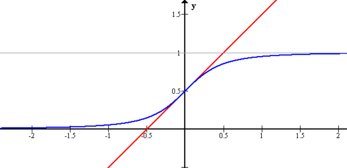
Logistic regression, contrary to the name, is a classification algorithm. Unlike linear regression which outputs a continuous value (e.g. house price) for the prediction, Logistic Regression transforms the output into a probability value (i.e. a number between 0 and 1) using what is known as the logistic sigmoid function. This function is also known as the squashing function since it maps a line — that can run from negative infinity to positive infinity along the y-axis — to a number between 0 and 1.
Here is what the graph of the sigmoid function looks like:
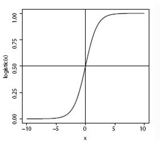
The function is called the sigmoid function because it is s-shaped. Here is what the sigmoid function looks like in mathematical notation:
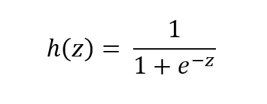
where:
- h(z) is the predicted probability of a given instance (i.e. example) being in the positive class…that is the class represented as 1 in a data set. For example, in an e-mail classification data set, this would be the probability that a given e-mail instance is spam (If h(z) = 0.73, for example, that would mean that the instance has a 73% chance of being spam).
- 1- h(z) is the probability of an instance being in the negative class, the class represented as 0 (e.g. not spam). h(z) is always a number between 0 and 1. Going back to the example in the bullet point above, this would mean that the instance has a 27% change of being not spam.
- z is the input (e.g. a weighted sum of the attributes of a given instance)
- e is Euler’s number
z is commonly expressed as the dot product, w · x, where w is a 1-dimensional vector containing the weights for each attribute, and x is a vector containing the values of each attribute for a specific instance of the data set (i.e. example).
Often the dot product, w · x, is written as matrix multiplication. In that case, z = wTx where T means transpose of the single dimensional weight vector w. The symbol Ɵ is often used in place of w.
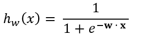
So substituting w · x into the sigmoid equation, we getthe following equation:

where
- w is a 1-dimensional vector containing the weights for each attribute.
- The subscript w on hw means the attributes x are weighted by the weight vector w.
- hw(x) is the probability (a value between 0 and 1) that an instance is a member of the positive class (i.e. probability an e-mail is spam).
- x is a vector containing the values of each attribute for a specific instance of the data set.
- w · x = w0x0 + w1x1
+ w2x2 + …. + wdxd (analogous to the equation of a line y
= mx + b from grade school)
- d is the number of attributes in the data set
- x0 = 1 by convention, for all instances. This attribute has to be added by the programmer for all instances. It is known formally as the “bias” term.
As is the case for many machine learning algorithms, the starting point for Logistic Regression is to create a trained model. One we have a trained model, we can use it to make predictions on new, unseen instances.
Training Phase
Creating a trained model entails determining the weight vector w. Once we have the weights, we can make predictions on new unseen examples. All we need are the values of the attributes of those examples (i.e. the x values), and we can weight the x values with the values of w to compute the probabilities h(x) for that example using the sigmoid function.
The rule for making predictions using the sigmoid function is as follows:
- If hw(x) ≥ 0.5, class = 1 (positive class, e.g. spam)
- If hw(x) < 0.5, class = 0 (negative class, e.g. not spam)
To determine the weights in linear regression, the sum of the squared error was the cost function (where error = actual values – predicted values by the line). The cost function represents how wrong a prediction is. In linear regression, it represents how wrong a line of best fit is on a set of observed training instances. The lower the sum of the squared error, the better a line fits the training data, and, in theory, the better the line will predict new, unseen instances.
Instead, the cost function in Logistic Regression is called cross-entropy. Without getting too detailed into the mathematics and notation of this particular equation, the cross-entropy equation is the one that we want to minimize. Minimizing this equation will yield us a sigmoid curve that best fits the training data and enables us to make the best classification predictions possible for new, unseen test instances. A minimum of the cost function is attained when the gradient of the cost function is close to zero (i.e. the calculated weights stop changing). The formal term for the gradient of the cost function getting close to zero is called convergence.
In order to minimize the cost function, we need to find its gradient (i.e. derivative, slope, etc.) and determine the values for the weight vector w that make its derivative as close to 0 as possible. We cannot just set the gradient to 0 and then enter x-values and calculate the weights directly. Instead, we have to use a method called gradient descent in order to find the weights.
In the gradient descent algorithm for Logistic Regression, we:
- Start off with an empty weight vector (initialized to random values between -0.01 and 0.01). The size of the vector is equal to the number of attributes in the data set.
- Initialize an empty weight change vector initialized to all zeros. The size of the vector is equal to the number of attributes in the data set.
- For each training instance, one at a time.
- a. Make a probability prediction by calculating the weighted sum of the attribute values and running that value through the sigmoid function.
- b. We evaluate the gradient of the cost function by plugging in the actual (i.e. observed) class value and the predicted class value from bullet point 3a above.
- c. The gradient value from 3b gets added to the weight change vector.
- After we finish with the last training instance from 3, we multiply each value in the weight change vector by a learning rate (commonly 0.01).
- The vector from 4 gets added to the empty weight vector to update the weights.
- We then ask two questions
- a. Have the weights continued to change (i.e. is the norm (i.e. magnitude) of the weight change vector less than a certain threshold like 0.001)?
- b. Have we been through the data set less than 10,000 (or whatever we set the maximum iterations to) times?
- c. If the answer is yes to both 6a and 6b, go back to step 2. Otherwise, we return the final weight vector, exiting the algorithm.
The gradient descent pseudocode for Logistic Regression is provided in Figure 10.6 of Introduction to Machine Learning by Ethem Alpaydin (Alpaydin, 2014).
Testing Phase
Once training is completed, we have the weights and can use these weights, attribute values, and the sigmoid function to make predictions for the set of test instances.
Predictions for a given test instance are made using the aforementioned sigmoid function:
Where the rule for making predictions using the sigmoid function is as follows:
- If hw(x) ≥ 0.5, class = 1 (positive class, e.g. spam)
- If hw(x) < 0.5, class = 0 (negative class, e.g. not spam)
Multi-class Logistic Regression
A Multi-class Logistic Regression problem is a twist on the binary Logistic Regression method presented above. Multi-class Logistic Regression can make predictions on both binary and multi-class classification problems.
In order to make predictions for multi-class datasets, we take the training set and create multiple separate binary classification problems (one for each class in the data set). For each of those training sets that we generated, we set the class values for one class to 1 (representing the positive class), and we set all other classes to 0 (i.e. the negative class).
In other words, if there are k classes in a data set, k separate training sets are generated. In each of those k separate training sets, one class is set to 1 and all other classes are set to 0.
In Multi-class Logistic Regression, the training phase entails creating k different weight vectors, one for each class rather than just a single weight vector (which was the case in binary Logistic Regression). Each weight vector will help to predict the probability of an instance being a member of that class. Thus, in the testing phase, when there is an unseen new instance, three different predictions need to be made. This method is called the one-vs-all strategy, sometimes called one-vs-rest.
The rule for making predictions for a given instance are as follows:
- For each new test instance,
- Make k separate probability predictions.
- Pick the class that has the highest probability (i.e. the class that is the most enthusiastic about that instance being a member of its class)
Other multi-class Logistic Regression algorithms include Softmax Regression and the one-vs-one strategy. The one-vs-all strategy was selected due to its popularity as being the default strategy used in practice for many of the well-known machine learning libraries for Python (Rebala, Ravi, & Churiwala, 2019)
Video
Here is an excellent video on logistic regression that explains the whole process I described above, step-by-step.
Logistic Regression Algorithm Design
The Logistic Regression algorithm was implemented from scratch. The Breast Cancer, Glass, Iris, Soybean (small), and Vote data sets were preprocessed to meet the input requirements of the algorithms. I used five-fold stratified cross-validation to evaluate the performance of the models.
Required Data Set Format for Logistic Regression
Columns (0 through N)
- 0: Instance ID
- 1: Attribute 1
- 2: Attribute 2
- 3: Attribute 3
- …
- N: Actual Class
The program then adds two additional columns for the testing set.
- N + 1: Predicted Class
- N + 2: Prediction Correct? (1 if yes, 0 if no)
Breast Cancer Data Set
This breast cancer data set contains 699 instances, 10 attributes, and a class – malignant or benign (Wolberg, 1992).
Modification of Attribute Values
The actual class value was changed to “Benign” or “Malignant.”
I transformed the attributes into binary numbers so that the algorithms could process the data properly and efficiently. If attribute value was greater than 5, the value was changed to 1, otherwise it was 0.
Missing Data
There were 16 missing attribute values, each denoted with a “?”. I chose a random number between 1 and 10 (inclusive) to fill in the data.
Glass Data Set
This glass data set contains 214 instances, 10 attributes, and 7 classes (German, 1987). The purpose of the data set is to identify the type of glass.
Modification of Attribute Values
If attribute values were greater than the median of the attribute, value was changed to 1, otherwise it was set to 0.
Missing Data
There are no missing values in this data set.
Iris Data Set
This data set contains 3 classes of 50 instances each (150 instances in total), where each class refers to a different type of iris plant (Fisher, 1988).
Modification of Attribute Values
If attribute values were greater than the median of the attribute, value was changed to 1, otherwise it was set to 0.
Missing Data
There were no missing attribute values.
Soybean Data Set (small)
This soybean (small) data set contains 47 instances, 35 attributes, and 4 classes (Michalski, 1980). The purpose of the data set is to determine the disease type.
Modification of Attribute Values
If attribute values were greater than the median of the attribute, value was changed to 1, otherwise it was set to 0.
Missing Data
There are no missing values in this data set.
Vote Data Set
This data set includes votes for each of the U.S. House of Representatives Congressmen (435 instances) on the 16 key votes identified by the Congressional Quarterly Almanac (Schlimmer, 1987). The purpose of the data set is to identify the representative as either a Democrat or Republican.
- 267 Democrats
- 168 Republicans
Modification of Attribute Values
I did the following modifications:
- Changed all “y” to 1 and all “n” to 0.
Missing Data
Missing values were denoted as “?”. To fill in those missing values, I chose random number, either 0 (“No”) or 1 (“Yes”).
Description of Any Tuning Process Applied
Some tuning was performed in this project. The learning rate was set to 0.01 by convention. A higher learning rate (0.5) resulted in poor results for the norm of the gradient (>1).
The stopping criteria for gradient descent was as follows:
- Maximum iterations = 10,000
- Euclidean norm of weight change vector < 0.001
When I tried max iterations at 100, the Euclidean norm of the weight change vector returned high values (> 0.2) which indicated that I needed to set a higher max iterations value in order to have a higher chance of convergence (i.e. weights stop changing) based on the norm stopping criteria.
Logistic Regression Algorithm in Python, Coded From Scratch
Here are the preprocessed data sets:
Here is the driver code. This is where the main method is located:
import pandas as pd # Import Pandas library
import numpy as np # Import Numpy library
import five_fold_stratified_cv
import logistic_regression

# File name: logistic_regression_driver.py
# Author: Addison Sears-Collins
# Date created: 7/19/2019
# Python version: 3.7
# Description: Driver of the logistic_regression.py program

# Required Data Set Format for Disrete Class Values
# Columns (0 through N)
# 0: Instance ID
# 1: Attribute 1
# 2: Attribute 2
# 3: Attribute 3
# ...
# N: Actual Class

# The logistic_regression.py program then adds 2 additional columns
# for the test set.
# N + 1: Predicted Class
# N + 2: Prediction Correct? (1 if yes, 0 if no)

ALGORITHM_NAME = "Logistic Regression"
SEPARATOR = ","  # Separator for the data set (e.g. "\t" for tab data)

def main():

    print("Welcome to the " +  ALGORITHM_NAME + " Program!")
    print()

    # Directory where data set is located
    data_path = input("Enter the path to your input file: ")
    #data_path = "iris.txt"

    # Read the full text file and store records in a Pandas dataframe
    pd_data_set = pd.read_csv(data_path, sep=SEPARATOR)

    # Show functioning of the program
    trace_runs_file = input("Enter the name of your trace runs file: ")
    #trace_runs_file = "iris_logistic_regression_trace_runs.txt"

    # Open a new file to save trace runs
    outfile_tr = open(trace_runs_file,"w")

    # Testing statistics
    test_stats_file = input("Enter the name of your test statistics file: ")
    #test_stats_file = "iris_logistic_regression_test_stats.txt"

    # Open a test_stats_file
    outfile_ts = open(test_stats_file,"w")

    # The number of folds in the cross-validation
    NO_OF_FOLDS = 5

    # Generate the five stratified folds
    fold0, fold1, fold2, fold3, fold4 = five_fold_stratified_cv.get_five_folds(
        pd_data_set)

    training_dataset = None
    test_dataset = None

    # Create an empty array of length 5 to store the accuracy_statistics
    # (classification accuracy)
    accuracy_statistics = np.zeros(NO_OF_FOLDS)

    # Run Logistic Regression the designated number of times as indicated by the
    # number of folds
    for experiment in range(0, NO_OF_FOLDS):

        print()
        print("Running Experiment " + str(experiment + 1) + " ...")
        print()
        outfile_tr.write("Running Experiment " + str(experiment + 1) + " ...\n")
        outfile_tr.write("\n")

        # Each fold will have a chance to be the test data set
        if experiment == 0:
            test_dataset = fold0
            training_dataset = pd.concat([
               fold1, fold2, fold3, fold4], ignore_index=True, sort=False)
        elif experiment == 1:
            test_dataset = fold1
            training_dataset = pd.concat([
               fold0, fold2, fold3, fold4], ignore_index=True, sort=False)
        elif experiment == 2:
            test_dataset = fold2
            training_dataset = pd.concat([
               fold0, fold1, fold3, fold4], ignore_index=True, sort=False)
        elif experiment == 3:
            test_dataset = fold3
            training_dataset = pd.concat([
               fold0, fold1, fold2, fold4], ignore_index=True, sort=False)
        else:
            test_dataset = fold4
            training_dataset = pd.concat([
               fold0, fold1, fold2, fold3], ignore_index=True, sort=False)

        accuracy, predictions, weights_for_each_class, no_of_instances_test = (
        logistic_regression.logistic_regression(training_dataset,test_dataset))

        # Print the trace runs of each experiment
        print("Accuracy:")
        print(str(accuracy * 100) + "%")
        print()
        print("Classifications:")
        print(predictions)
        print()
        print("Learned Model:")
        print(weights_for_each_class)
        print()
        print("Number of Test Instances:")
        print(str(no_of_instances_test))
        print()

        outfile_tr.write("Accuracy:")
        outfile_tr.write(str(accuracy * 100) + "%\n\n")
        outfile_tr.write("Classifications:\n")
        outfile_tr.write(str(predictions) + "\n\n")
        outfile_tr.write("Learned Model:\n")
        outfile_tr.write(str(weights_for_each_class) + "\n\n")
        outfile_tr.write("Number of Test Instances:")
        outfile_tr.write(str(no_of_instances_test) + "\n\n")

        # Store the accuracy in the accuracy_statistics array
        accuracy_statistics[experiment] = accuracy

    outfile_tr.write("Experiments Completed.\n")
    print("Experiments Completed.\n")

    # Write to a file
    outfile_ts.write("----------------------------------------------------------\n")
    outfile_ts.write(ALGORITHM_NAME + " Summary Statistics\n")
    outfile_ts.write("----------------------------------------------------------\n")
    outfile_ts.write("Data Set : " + data_path + "\n")
    outfile_ts.write("\n")
    outfile_ts.write("Accuracy Statistics for All 5 Experiments:")
    outfile_ts.write(np.array2string(
        accuracy_statistics, precision=2, separator=',',
        suppress_small=True))
    outfile_ts.write("\n")
    outfile_ts.write("\n")
    accuracy = np.mean(accuracy_statistics)
    accuracy *= 100
    outfile_ts.write("Classification Accuracy : " + str(accuracy) + "%\n")

    # Print to the console
    print()
    print("----------------------------------------------------------")
    print(ALGORITHM_NAME + " Summary Statistics")
    print("----------------------------------------------------------")
    print("Data Set : " + data_path)
    print()
    print()
    print("Accuracy Statistics for All 5 Experiments:")
    print(accuracy_statistics)
    print()
    print()
    print("Classification Accuracy : " + str(accuracy) + "%")
    print()

    # Close the files
    outfile_tr.close()
    outfile_ts.close()

main()
Here is the code for logistic regression:
import pandas as pd # Import Pandas library
import numpy as np # Import Numpy library

# File name: logistic_regression.py
# Author: Addison Sears-Collins
# Date created: 7/19/2019
# Python version: 3.7
# Description: Multi-class logistic regression using one-vs-all.

# Required Data Set Format for Disrete Class Values
# Columns (0 through N)
# 0: Instance ID
# 1: Attribute 1
# 2: Attribute 2
# 3: Attribute 3
# ...
# N: Actual Class

# This program then adds 2 additional columns for the test set.
# N + 1: Predicted Class
# N + 2: Prediction Correct? (1 if yes, 0 if no)

def sigmoid(z):
    """
    Parameters:
        z: A real number
    Returns:
        1.0/(1 + np.exp(-z))
    """
    return 1.0/(1 + np.exp(-z))

def gradient_descent(training_set):
    """
    Gradient descent for logistic regression. Follows method presented
    in the textbook Introduction to Machine Learning 3rd Edition by
    Ethem Alpaydin (pg. 252)

    Parameters:
      training_set: The training instances as a Numpy array
    Returns:
      weights: The vector of weights, commonly called w or THETA
    """

    no_of_columns_training_set = training_set.shape[1]
    no_of_rows_training_set = training_set.shape[0]

    # Extract the attributes from the training set.
    # x is still a 2d array
    x = training_set[:,:(no_of_columns_training_set - 1)]
    no_of_attributes = x.shape[1]

    # Extract the classes from the training set.
    # actual_class is a 1d array.
    actual_class = training_set[:,(no_of_columns_training_set - 1)]

    # Set a learning rate
    LEARNING_RATE = 0.01

    # Set the maximum number of iterations
    MAX_ITER = 10000

    # Set the iteration variable to 0
    iter = 0

    # Set a flag to determine if we have exceeded the maximum number of
    # iterations
    exceeded_max_iter = False

    # Set the tolerance. When the euclidean norm of the gradient vector
    # (i.e. magnitude of the changes in the weights) gets below this value,
    # stop iterating through the while loop
    GRAD_TOLERANCE = 0.001
    norm_of_gradient = None

    # Set a flag to determine if we have reached the minimum of the
    # cost (i.e. error) function.
    converged = False

    # Create the weights vector with random floats between -0.01 and 0.01
    # The number of weights is equal to the number of attributes
    weights = np.random.uniform(-0.01,0.01,(no_of_attributes))
    changes_in_weights = None

    # Keep running the loop below until convergence on the minimum of the
    # cost function or we exceed the max number of iterations
    while(not(converged) and not(exceeded_max_iter)):

        # Initialize a weight change vector that stores the changes in
        # the weights at each iteration
        changes_in_weights = np.zeros(no_of_attributes)

        # For each training instance
        for inst in range(0, no_of_rows_training_set):

            # Calculate weighted sum of the attributes for
            # this instance
            output = np.dot(weights, x[inst,:])

            # Calculate the sigmoid of the weighted sum
            # This y is the probability that this instance belongs
            # to the positive class
            y =  sigmoid(output)

            # Calculate difference
            difference = (actual_class[inst] - y)

            # Multiply the difference by the attribute vector
            product = np.multiply(x[inst,:], difference)

            # For each attribute, update the weight changes
            # i.e. the gradient vector
            changes_in_weights = np.add(changes_in_weights,product)

        # Calculate the step size
        step_size = np.multiply(changes_in_weights, LEARNING_RATE)

        # Update the weights vector
        weights = np.add(weights, step_size)

        # Test to see if we have converged on the minimum of the error
        # function
        norm_of_gradient = np.linalg.norm(changes_in_weights)

        if (norm_of_gradient < GRAD_TOLERANCE):
            converged = True

        # Update the number of iterations
        iter += 1

        # If we have exceeded the maximum number of iterations
        if (iter > MAX_ITER):
            exceeded_max_iter = True

    #For debugging purposes
    #print("Number of Iterations: " + str(iter - 1))
    #print("Norm of the gradient: " + str(norm_of_gradient))
    #print(changes_in_weights)
    #print()
    return weights


def logistic_regression(training_set, test_set):
    """
    Multi-class one-vs-all logistic regression
    Parameters:
      training_set: The training instances as a Pandas dataframe
      test_set: The test instances as a Pandas dataframe
    Returns:
      accuracy: Classification accuracy as a decimal
      predictions: Classifications of all the test instances as a
        Pandas dataframe
      weights_for_each_class: The weight vectors for each class (one-vs-all)
      no_of_instances_test: The number of test instances
    """

    # Remove the instance ID column
    training_set = training_set.drop(
        training_set.columns[[0]], axis=1)
    test_set = test_set.drop(
        test_set.columns[[0]], axis=1)

    # Make a list of the unique classes
    list_of_unique_classes = pd.unique(training_set["Actual Class"])

    # Replace all the class values with numbers, starting from 0
    # in both the test and training sets.
    for cl in range(0, len(list_of_unique_classes)):
        training_set["Actual Class"].replace(
            list_of_unique_classes[cl], cl ,inplace=True)
        test_set["Actual Class"].replace(
            list_of_unique_classes[cl], cl ,inplace=True)

    # Insert a column of 1s in column 0 of both the training
    # and test sets. This is the bias and helps with gradient
    # descent. (i.e. X0 = 1 for all instances)
    training_set.insert(0, "Bias", 1)
    test_set.insert(0, "Bias", 1)

    # Convert dataframes to numpy arrays
    np_training_set = training_set.values
    np_test_set = test_set.values

    # Add 2 additional columns to the testing dataframe
    test_set = test_set.reindex(
        columns=[*test_set.columns.tolist(
        ), 'Predicted Class', 'Prediction Correct?'])

    ############################# Training Phase ##############################

    no_of_columns_training_set = np_training_set.shape[1]
    no_of_rows_training_set = np_training_set.shape[0]

    # Create and store a training set for each unique class
    # to create separate binary classification
    # problems
    trainingsets = []
    for cl in range(0, len(list_of_unique_classes)):

        # Create a copy of the training set
        temp = np.copy(np_training_set)

        # This class becomes the positive class 1
        # and all other classes become the negative class 0
        for row in range(0, no_of_rows_training_set):
            if (temp[row, (no_of_columns_training_set - 1)]) == cl:
                temp[row, (no_of_columns_training_set - 1)] = 1
            else:
                temp[row, (no_of_columns_training_set - 1)] = 0

        # Add the new training set to the trainingsets list
        trainingsets.append(temp)

    # Calculate and store the weights for the training set
    # of each class. Execute gradient descent on each training set
    # in order to calculate the weights
    weights_for_each_class = []

    for cl in range(0, len(list_of_unique_classes)):
        weights_for_this_class = gradient_descent(trainingsets[cl])
        weights_for_each_class.append(weights_for_this_class)

    # Used for debugging
    #print(weights_for_each_class[0])
    #print()
    #print(weights_for_each_class[1])
    #print()
    #print(weights_for_each_class[2])

    ########################### End of Training Phase #########################

    ############################# Testing Phase ###############################

    no_of_columns_test_set = np_test_set.shape[1]
    no_of_rows_test_set = np_test_set.shape[0]

    # Extract the attributes from the test set.
    # x is still a 2d array
    x = np_test_set[:,:(no_of_columns_test_set - 1)]
    no_of_attributes = x.shape[1]

    # Extract the classes from the test set.
    # actual_class is a 1d array.
    actual_class = np_test_set[:,(no_of_columns_test_set - 1)]

    # Go through each row (instance) of the test data
    for inst in range(0,  no_of_rows_test_set):

        # Create a scorecard that keeps track of the probabilities of this
        # instance being a part of each class
        scorecard = []

        # Calculate and store the probability for each class in the scorecard
        for cl in range(0, len(list_of_unique_classes)):

            # Calculate weighted sum of the attributes for
            # this instance
            output = np.dot(weights_for_each_class[cl], x[inst,:])

            # Calculate the sigmoid of the weighted sum
            # This is the probability that this instance belongs
            # to the positive class
            this_probability = sigmoid(output)

            scorecard.append(this_probability)

        most_likely_class = scorecard.index(max(scorecard))

        # Store the value of the most likely class in the "Predicted Class"
        # column of the test_set data frame
        test_set.loc[inst, "Predicted Class"] = most_likely_class

        # Update the 'Prediction Correct?' column of the test_set data frame
        # 1 if correct, else 0
        if test_set.loc[inst, "Actual Class"] == test_set.loc[
            inst, "Predicted Class"]:
            test_set.loc[inst, "Prediction Correct?"] = 1
        else:
            test_set.loc[inst, "Prediction Correct?"] = 0

    # accuracy = (total correct predictions)/(total number of predictions)
    accuracy = (test_set["Prediction Correct?"].sum())/(len(test_set.index))

    # Store the revamped dataframe
    predictions = test_set

    # Replace all the class values with the name of the class
    for cl in range(0, len(list_of_unique_classes)):
        predictions["Actual Class"].replace(
            cl, list_of_unique_classes[cl] ,inplace=True)
        predictions["Predicted Class"].replace(
            cl, list_of_unique_classes[cl] ,inplace=True)

    # Replace 1 with Yes and 0 with No in the 'Prediction
    # Correct?' column
    predictions['Prediction Correct?'] = predictions[
        'Prediction Correct?'].map({1: "Yes", 0: "No"})

    # Reformat the weights_for_each_class list of arrays
    weights_for_each_class = pd.DataFrame(np.row_stack(weights_for_each_class))

    # Rename the row names
    for cl in range(0, len(list_of_unique_classes)):
        row_name = str(list_of_unique_classes[cl] + " weights")
        weights_for_each_class.rename(index={cl:row_name}, inplace=True)

    # Get a list of the names of the attributes
    training_set_names = list(training_set.columns.values)
    training_set_names.pop() # Remove 'Actual Class'

    # Rename the column names
    for col in range(0, len(training_set_names)):
        col_name = str(training_set_names[col])
        weights_for_each_class.rename(columns={col:col_name}, inplace=True)

    # Record the number of test instances
    no_of_instances_test = len(test_set.index)

    # Return statement
    return accuracy, predictions, weights_for_each_class, no_of_instances_test
Here is the code for five-fold stratified cross-validation:
import pandas as pd # Import Pandas library
import numpy as np # Import Numpy library

# File name: five_fold_stratified_cv.py
# Author: Addison Sears-Collins
# Date created: 7/17/2019
# Python version: 3.7
# Description: Implementation of five-fold stratified cross-validation
# Divide the data set into five random groups. Make sure
# that the proportion of each class in each group is roughly equal to its
# proportion in the entire data set.

# Required Data Set Format for Disrete Class Values
# Columns (0 through N)
# 0: Instance ID
# 1: Attribute 1
# 2: Attribute 2
# 3: Attribute 3
# ...
# N: Actual Class

def get_five_folds(instances):
    """
    Parameters:
        instances: A Pandas data frame containing the instances
    Returns:
        fold0, fold1, fold2, fold3, fold4
        Five folds whose class frequency distributions are
        each representative of the entire original data set (i.e. Five-Fold
        Stratified Cross Validation)
    """
    # Shuffle the data set randomly
    instances = instances.sample(frac=1).reset_index(drop=True)

    # Record the number of columns in the data set
    no_of_columns = len(instances.columns) # number of columns

    # Record the number of rows in the data set
    no_of_rows = len(instances.index) # number of rows

    # Create five empty folds (i.e. Panda Dataframes: fold0 through fold4)
    fold0 = pd.DataFrame(columns=(instances.columns))
    fold1 = pd.DataFrame(columns=(instances.columns))
    fold2 = pd.DataFrame(columns=(instances.columns))
    fold3 = pd.DataFrame(columns=(instances.columns))
    fold4 = pd.DataFrame(columns=(instances.columns))

    # Record the column of the Actual Class
    actual_class_column = no_of_columns - 1

    # Generate an array containing the unique
    # Actual Class values
    unique_class_list_df = instances.iloc[:,actual_class_column]
    unique_class_list_df = unique_class_list_df.sort_values()
    unique_class_list_np = unique_class_list_df.unique() #Numpy array
    unique_class_list_df = unique_class_list_df.drop_duplicates()#Pandas df

    unique_class_list_np_size = unique_class_list_np.size

    # For each unique class in the unique Actual Class array
    for unique_class_list_np_idx in range(0, unique_class_list_np_size):

        # Initialize the counter to 0
        counter = 0

        # Go through each row of the data set and find instances that
        # are part of this unique class. Distribute them among one
        # of five folds
        for row in range(0, no_of_rows):

            # If the value of the unique class is equal to the actual
            # class in the original data set on this row
            if unique_class_list_np[unique_class_list_np_idx] == (
                instances.iloc[row,actual_class_column]):

                    # Allocate instance to fold0
                    if counter == 0:

                        # Extract data for the new row
                        new_row = instances.iloc[row,:]

                        # Append that entire instance to fold
                        fold0.loc[len(fold0)] = new_row

                        # Increase the counter by 1
                        counter += 1

                    # Allocate instance to fold1
                    elif counter == 1:

                        # Extract data for the new row
                        new_row = instances.iloc[row,:]

                        # Append that entire instance to fold
                        fold1.loc[len(fold1)] = new_row

                        # Increase the counter by 1
                        counter += 1

                    # Allocate instance to fold2
                    elif counter == 2:

                        # Extract data for the new row
                        new_row = instances.iloc[row,:]

                        # Append that entire instance to fold
                        fold2.loc[len(fold2)] = new_row

                        # Increase the counter by 1
                        counter += 1

                    # Allocate instance to fold3
                    elif counter == 3:

                        # Extract data for the new row
                        new_row = instances.iloc[row,:]

                        # Append that entire instance to fold
                        fold3.loc[len(fold3)] = new_row

                        # Increase the counter by 1
                        counter += 1

                    # Allocate instance to fold4
                    else:

                        # Extract data for the new row
                        new_row = instances.iloc[row,:]

                        # Append that entire instance to fold
                        fold4.loc[len(fold4)] = new_row

                        # Reset counter to 0
                        counter = 0

    return fold0, fold1, fold2, fold3, fold4
Logistic Regression Output
Here are the trace runs:
Here are the results:
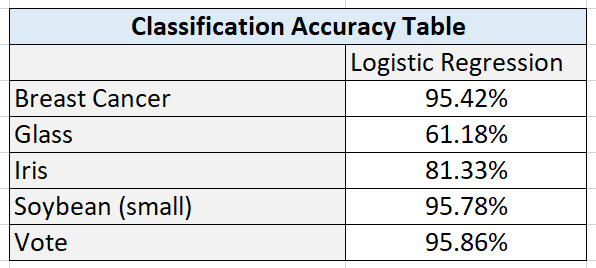
Here are the test statistics for each data set:
Analysis
Breast Cancer Data Set
I hypothesize that performance was high on this algorithm because of the large number of instances (699 in total). This data set had the highest number of instances out of all the data sets.
These results also suggest that the amount of training data has a direct impact on performance. Higher amounts of data can lead to better learning and better classification accuracy on new, unseen instances.
Glass Data Set
I hypothesize that the poor performance on the glass data set is due to the high numbers of classes combined with a relatively smaller data set.
Iris Data Set
Classification accuracy on the iris data set was satisfactory. This data set was small, and more training data would be needed to see if accuracy could be improved by giving the algorithm more data to learn the underlying relationship between the attributes and the flower types.
Soybean Data Set (small)
I hypothesize that the large numbers of attributes in the soybean data set (35) helped balance the relatively small number of training instances. These results suggest that large numbers of relevant attributes can help a machine learning algorithm create more accurate classifications.
Vote Data Set
The results show that classification algorithms like Logistic Regression can have outstanding performance on large data sets that are binary classification problems.
Summary and Conclusions
- Higher amounts of data can lead to better learning and better classification accuracy on new, unseen instances.
- Large numbers of relevant attributes can help a machine learning algorithm create more accurate classifications.
- Classification algorithms like Logistic Regression can achieve excellent classification accuracy on binary classification problems, but performance on multi-class classification algorithms can yield mixed results.
References
Alpaydin, E. (2014). Introduction to Machine Learning. Cambridge, Massachusetts: The MIT Press.
Fisher, R. (1988, July 01). Iris Data Set. Retrieved from Machine Learning Repository: https://archive.ics.uci.edu/ml/datasets/iris
German, B. (1987, September 1). Glass Identification Data Set. Retrieved from UCI Machine Learning Repository: https://archive.ics.uci.edu/ml/datasets/Glass+Identification
Kelleher, J. D., Namee, B., & Arcy, A. (2015). Fundamentals of Machine Learning for Predictive Data Analytics. Cambridge, Massachusetts: The MIT Press.
Michalski, R. (1980). Learning by being told and learning from examples: an experimental comparison of the two methodes of knowledge acquisition in the context of developing an expert system for soybean disease diagnosis. International Journal of Policy Analysis and Information Systems, 4(2), 125-161.
Rebala, G., Ravi, A., & Churiwala, S. (2019). An Introduction to Machine Learning. Switzerland: Springer.
Schlimmer, J. (1987, 04 27). Congressional Voting Records Data Set. Retrieved from Machine Learning Repository: https://archive.ics.uci.edu/ml/datasets/Congressional+Voting+Records
Wolberg, W. (1992, 07 15). Breast Cancer Wisconsin (Original) Data Set. Retrieved from Machine Learning Repository: https://archive.ics.uci.edu/ml/datasets/Breast+Cancer+Wisconsin+%28Original%25
Y. Ng, A., & Jordan, M. (2001). On Discriminative vs. Generative Classifiers: A Comparison of Logistic Regression and Naive Bayes. NIPS’01 Proceedings of the 14th International Conference on Neural Information Processing Systems: Natural and Synthetic , 841-848.