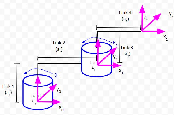
A kinematic diagram shows how the links (the stiff parts of the robot) and joints (the servo motors or linear actuators) are connected when each joint is at an angle of 0 degrees (or in its 0 position in the case of a linear actuator).
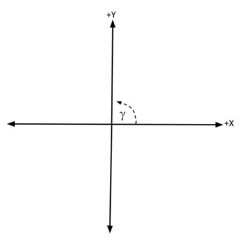
Remember that degree angles are measured in the counterclockwise direction, starting from the positive x-axis (see figure below).
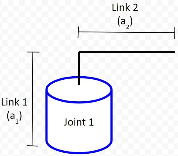
First, let’s start with creating our joint (revolute joint…i.e. the servo motor) as well as the two links. We’ll use the letter a to represent link lengths.
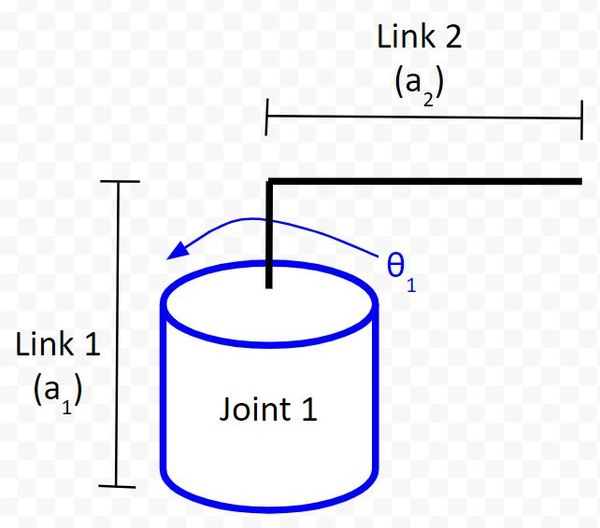
We now need to label the joint with the direction of positive rotation.
We use the right-hand rule whereby your thumb points in the direction of the rotation axis. In this case, your thumb will point upward (towards the ceiling) out of the servo horn. Your fingers will curl in the direction of positive rotation.
In this case, θ1 shows that the direction of positive rotation is counterclockwise if you are looking downward on the servo horn from above.
Add a Joint and a Link
Now, let’s add a joint (i.e. servo motor) to the end of link 2.
Remember, we will draw the diagram assuming that each joint is at 0 degrees.
We added another joint (i.e. a revolute joint because the motion entails revolution around a single axis) in the previous section.
Using the right-hand rule, take your thumb and point it in the direction of the axis of rotation (i.e. out of the top-center of the servo motor. Your fingers curl in the direction of positive rotation (in this case, counterclockwise…Note that clockwise rotation would be negative rotation).
Let’s draw the positive rotation.
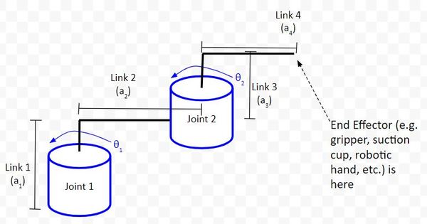
At this stage, our robotic arm (i.e. “manipulator”) has two degrees of freedom (2 DOF), corresponding to the two servo motors. The end effector would be the end of Link 4.
In robotics, an end effector is the part of the robot that has an effect on the outside world.
There are a lot of different types of robotic manipulator end effectors. An end effector could also be a gripper, suction cup, paint sprayer, etc.
References
Credit to Professor Angela Sodemann for teaching me this stuff. Dr. Sodemann is an excellent teacher (She runs a course on RoboGrok.com). On her YouTube channel, she provides some of the clearest explanations on robotics fundamentals you’ll ever hear.
In this section, we’ll take a look at how to build a two degree of freedom robotic arm. The robot we’ll develop will be an early prototype of a SCARA robot.
Special shout out to Professor Angela Sodemann for this project idea. She is an excellent teacher (She runs a course on RoboGrok.com). While she uses the PSoC in her work, I use Arduino since I’m more comfortable with this platform. Angela is an excellent teacher and does a fantastic job explaining various robotics topics over on her YouTube channel.
Real-World Applications
A SCARA robot packaging cookies into trays. Photo Credit: Gfycat.
SCARA robots are popular in small-scale manufacturing and logistics applications. They are some of the fastest and cheapest robots for pick and place tasks (picking up an object in one location and placing it in another). You can find lots of videos on the Internet showing SCARA robots in action.
The motors we’ll use in this project have a range from 0 to 180 degrees. We want to be able to send commands to the robotic arm so that the servos move to specific angles within this range. This project will be used in my future tutorials on forward kinematics and inverse kinematics.
Forward kinematics asks the question: Where is the end effector of a robot (e.g. gripper, hand, vacuum suction cup, etc.) located in space given that we know the angles of the servo motors? The opposite of forward kinematics is inverse kinematics.
Inverse kinematics asks, what should the angles of the servo motors be if we want the end effector to be located at a particular point in space? In a future tutorial, we’ll also learn about inverse kinematics.
Prerequisites
You have the Arduino IDE (Integrated Development Environment) installed on either your PC (Windows, MacOS, or Linux) or within a Virtual Box.
6 Channel Digital Servo Tester (available at AliExpress.com or eBay)
Actuonix L16 Linear Actuator 100mm 150:1 6V RC Control (available on eBay)
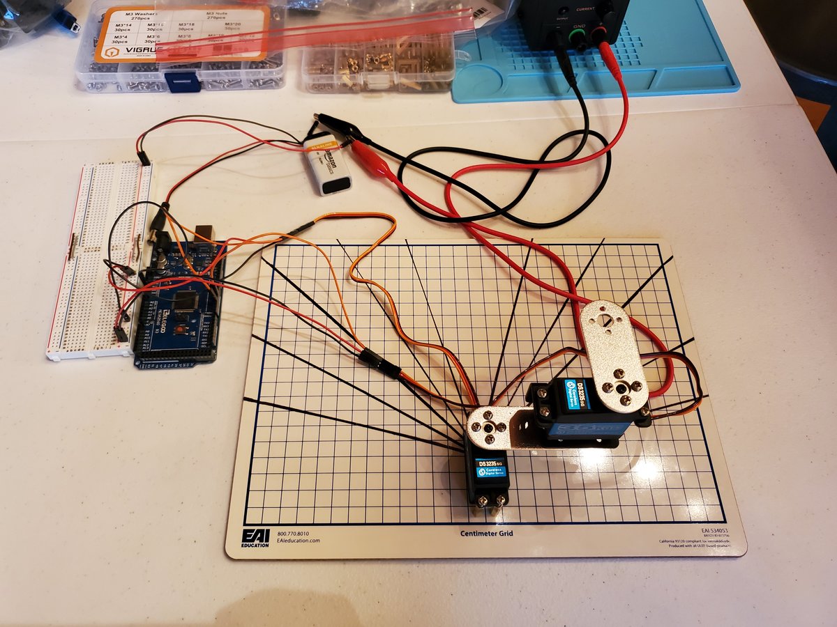
Set Up the Initial Hardware
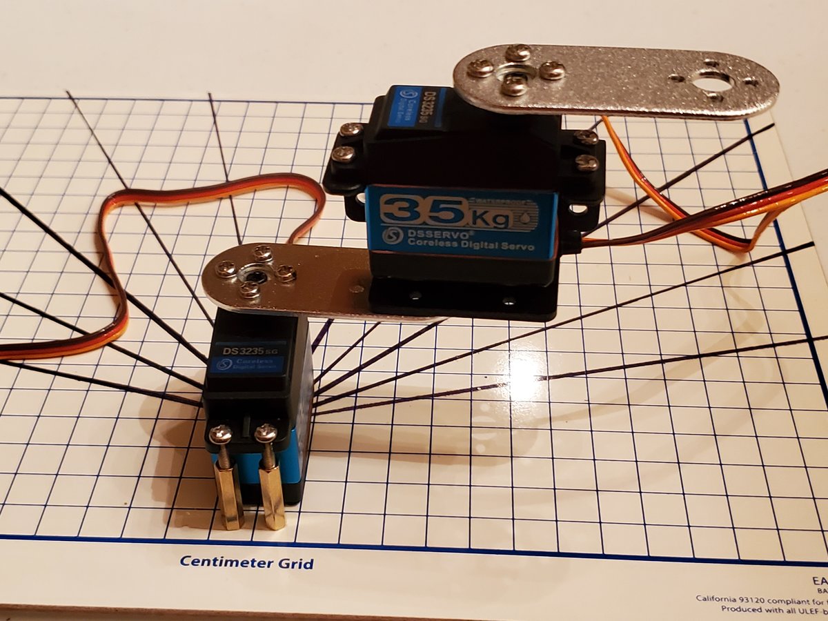
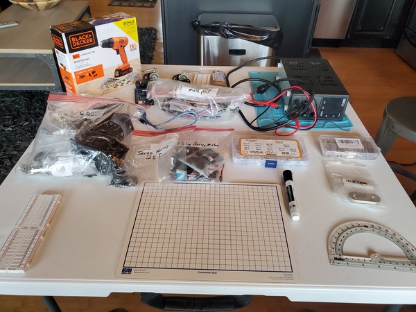
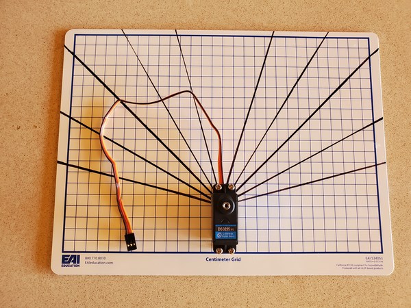
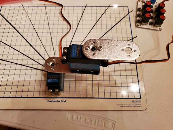
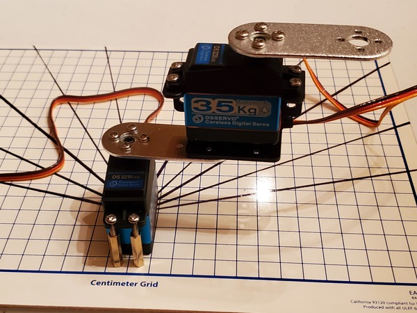
Lay out all the parts out on the table like this:
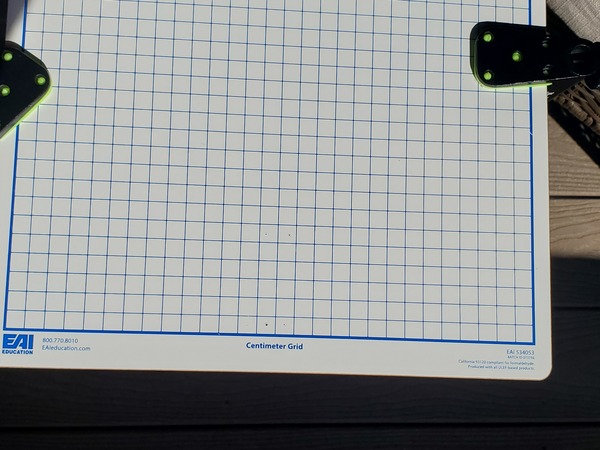
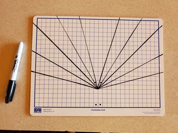
Grab your centimeter grid dry erase board and the two C-clamps.
Clamp down the dry erase board on a hard surface, like a table.
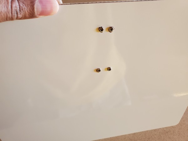
Mark four holes on the dry erase board using a screwdriver or some other sharp object.
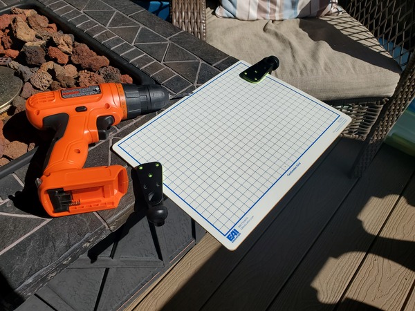
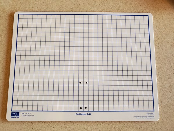
Using the drill, make four 3MM diameter holes like this.
Draw 10 lines on your board…5 lines on one side and 5 lines on the other side. Each line needs to be 15 degrees apart (use the protractor to measure the angle).
You can use some tape and a permanent marker to make sure the lines are permanently on there and are straight.
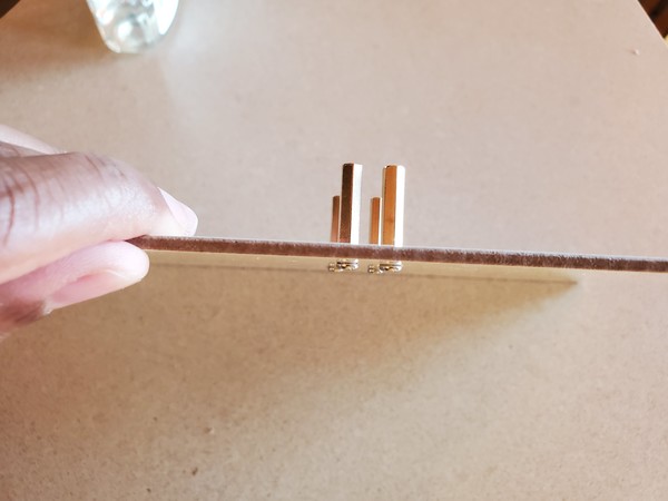
Grab four M3 x 10mm screws.
Put the screws up through the bottom of the board via the holes.
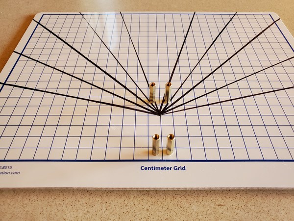
Grab four 20mm standoffs and screw them on top of the screws.
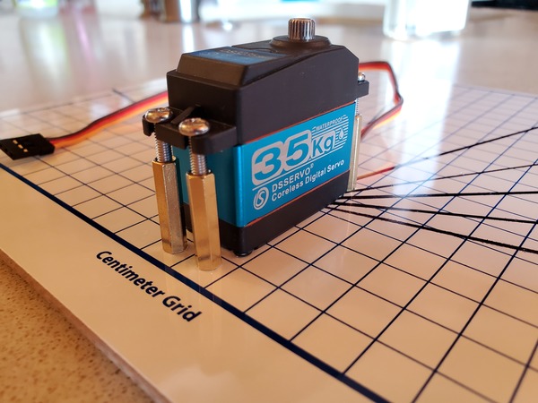
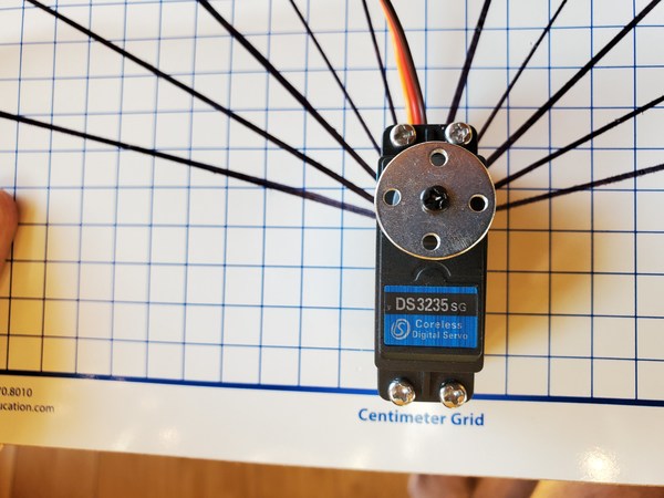
Take one 35kg servo motor and place it on top of the standoffs.
Grab four 20mm M3 screws and use these screws to secure the servo motor into the standoffs. The screws don’t need to be super tight…just tight enough so that the servo stays in one place.
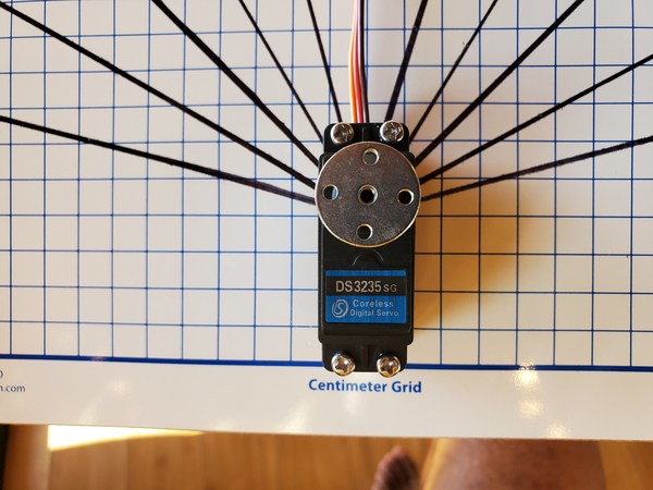
Grab a servo horn and attach it to the servo gear.
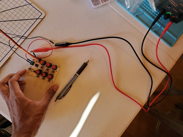
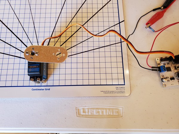
Grab the 6 Channel Digital Servo Tester and either a DC Variable Power Supply or 4 AA Batteries with Battery holder.
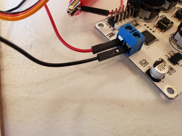
Plug the negative (black) lead of the power supply into the negative (-) socket of the 6 Channel Digital Servo Tester. I connected the black alligator clip coming from the power supply to a male-to-male jumper wire. You will have to unscrew the screw in the blue dongle from the top, and then slip the male-to-male jumper wire in the bottom. Then retighten the screw.
Plug the positive (red) lead of the power supply into the positive (+) socket of the 6 Channel Digital Servo Tester.
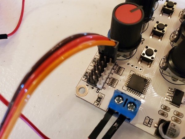
Plug the servo motor into one of the 3 header pin units on top of the 6 Channel Digital Servo Tester. The yellow wire should plug into S, red wire should plug into positive (+), and brown wire should plug into negative (-).
Turn on the DC power supply and set the voltage to 6V and the current limit to 1A.
Using the corresponding knob on the Digital Servo Tester, Rotate the servo horn as far as it can go in the clockwise direction. This is the 0 degree position (Note: if you press the little button under the knob, the servo will go to the 90 degree (center) position).
Take the servo horn off.
Place the servo horn back on the servo gear so that the two holes on either side of the servo horn are just a bit beyond perfectly horizontal.
Grab a servo screw and secure the servo horn on to the servo gear.
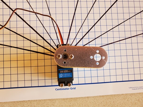
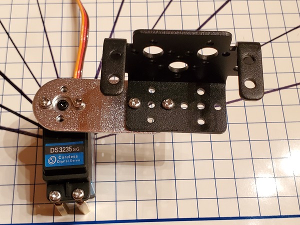
Grab a beam mount.
Attach the beam mount (i.e. robot arm “link”) to the servo horn using two small M3 x 4mm screws.
This motor, Joint 1 (also known as Servo 0), is now calibrated and complete. If you want to, you can add two more screws to the servo horn so that there are 4 screws that secure the beam mount to the servo horn.
Now, let’s add the second servo motor. We’ll call this second joint Servo 1.
Grab a multi-functional servo bracket.
Grab two M3 x 6mm screws and two M3 nuts.
Secure the multi-functional servo bracket into the beam mount.
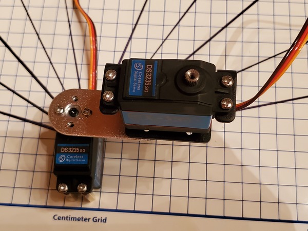
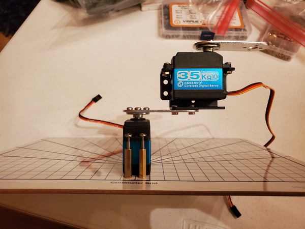
Grab a 35kg servo and place it into the multi-functional servo bracket.
Grab four M3 x 8mm screws and four M3 nuts.
Secure the servo into the multi-functional servo bracket.
Grab a servo horn, and place it on the gear of the servo.
Secure the servo horn with a servo screw.
Grab a beam mount and two M3 x 4mm screws. Secure the beam mount to the servo horn.
Place the three pins of this second servo into the corresponding pins of the 6 Channel Digital Servo Tester.
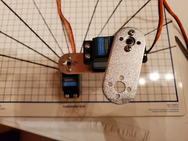
Adjust the position of the beam mount so that when the servo is in the middle of its range, the beam mount points straight to the right (i.e. when you press the center button under the corresponding knob on the 6 Channel Digital Servo Tester, the beam mount should point straight to the right).
Once you’re happy with the alignment, use two M3 x 4mm screws to secure the beam mount to the horn even further.
Our robotic arm now has the following components (two joints and four links):
Joint 1 – The bottom servo motor (goes from 0 degrees to 180 degrees).
Link 1 – Extends from the top of the dry erase board to the top of the servo horn of Joint 0.
Link 2 – Extends from the middle of the servo horn of Joint 1 to the end of the beam mount (i.e. specifically, to the center of the big central circle on the end of the beam mount).
Joint 2 – The top servo motor (goes from -90 degrees to 90 degrees…I’ll explain why we define the angle range like this when we learn about drawing kinematic diagrams in a future tutorial).
Link 3 – Extends from the beam mount to the top of the servo horn of Joint 2.
Link 4 – Extends from the middle of the servo horn of Joint 2 to the end of the beam mount
Here is the kinematic diagram for this robot. Don’t worry if you don’t understand it. We’ll learn how to create this in a future post.
Move Servos
In this section, we’ll get the servos moving. We’ll use the setup in the kinematic diagram above.
Turn on your DC power supply and set it to 6V with a 2A current limit (i.e. 1A per servo).
Plug the red and black leads of the power supply into the red and blue power rails of the breadboard. If you’re using 4xAA batteries, you can plug the leads into the breadboard now.
Write the Code for the Arduino Mega
Write the following code and load it to your Arduino. This code sweeps the two servos 180 degrees, going from the most clockwise position to the most counterclockwise position over and over again.
/*
Program: Sweep 2 Servos Using Arduino
File: sweep_servos_2dof.ino
Description: This program sweeps two servos (i.e. joints) 180 degrees, going from
  the most clockwise position to the most counterclockwise position.
  Note that Servo 0 = Joint 1 and Servo 1 = Joint 2.
Author: Addison Sears-Collins
Website: https://automaticaddison.com
Date: August 16, 2020
*/

#include <VarSpeedServo.h>

// Define the number of servos
#define SERVOS 2

// Create the servo objects.
VarSpeedServo myservo[SERVOS];

// Speed of the servo motors
// Speed=1: Slowest
// Speed=255: Fastest.
const int desired_speed = 75;

// Attach servos to digital pins on the Arduino
int servo_pins[SERVOS] = {3,5};

void setup() {

  // Attach the servos to the servo object
  // attach(pin, min, max  ) - Attaches to a pin
  //   setting min and max values in microseconds
  //   default min is 544, max is 2400
  // Alter these numbers until both servos have a
  //   180 degree range.
  myservo[0].attach(servo_pins[0], 544, 2475);
  myservo[1].attach(servo_pins[1], 500, 2475);

  // Set initial servo positions
  myservo[0].write(0, desired_speed, true);
  myservo[1].write(calc_servo_1_angle(90), desired_speed, true);

  // Wait one second to let servos get into position
  delay(1000);
}

void loop() {

    // To most counterclockwise position
    myservo[0].write(180, desired_speed, true);

    // Go to clockwise position
    myservo[1].write(calc_servo_1_angle(-90), desired_speed, true);

    // Go to counterclockwise position
    myservo[1].write(calc_servo_1_angle(90), desired_speed, true);

    // To most clockwise position
    myservo[0].write(0, desired_speed, true);

    // Wait half a second
    delay(500);
}

/*  This method converts the desired angle for Servo 1 into a control angle
 *  for Servo 1. It assumes that the 0 degree position on the kinematic
 *  diagram for Servo 1 is actually 90 degrees on the actual servo.
 *  The angle range for Servo 1 on the kinematic diagram is
 *  -90 to 90 degrees, with 0 degrees being the center position.
 *  The actual servo range for the physical motor
 *  is 0 to 180 degrees. We convert the desired angle
 *  to a value within that range.
 */
int calc_servo_1_angle (int input_angle) {

  int result;

  result = map(input_angle, -90, 90, 0, 180);

  return result;
}
Sweep and Calibrate the Servos
Run the code so that your servos start moving. Servo 0 (i.e. Joint 1) will rotate counterclockwise from 0 degrees to 180 degrees, then Servo 1 (i.e. Joint 2) will rotate clockwise from 90 degrees to -90 degrees. Then Servo 0 will rotate clockwise, back to the 0 degree position where it started.
You should see the same motion as in the animated gif image at the beginning of this tutorial.
You need to calibrate the servos so that the servos are aligned with the 0 degrees (i.e. +x axis) and 180 degrees (-x axis) on the dry erase board. In order to do that, you need to alter the minimum value of 544 microseconds and/or maximum value of 2400 microseconds of the pulse width for each servo until you align with the axes on the board. I recommend starting with the first servo (i.e. servo 0 which is attached to the board), and then calibrate the second servo (i.e. servo 1).
As the robotic arm sweeps back and forth, you see that the end-effector (the top beam mount) changes position (x and y coordinate) and orientation (i.e. the angle that the end-effector makes with the positive x-axis).
Position + orientation are known collectively as pose.
With a robotic arm, it is not enough to know where the end of the robotic arm (e.g. gripper) is located in space via its x, y, and z coordinates…you also need to know the direction the end of the robotic arm is pointing towards (i.e. orientation).
Consider, for example, a robotic arm with a paint sprayer at the end. We want the robotic arm to paint a car. We need to direct the arm to the appropriate position, and we need to make sure the angle of the arm is oriented in a way that directs the sprayer towards the place on the car’s surface you want to paint.
In a future post, we will learn how to calculate the position and orientation of a robotic arm, so stay tuned!
Kinematics is about how you convert the position and velocity of an end effector (e.g. gripper, robotic hand, etc.) to position and velocity of the joints (i.e. the servo motors along a robotic arm), and vice-versa.
Let’s take a look at the vocabulary of that sentence.
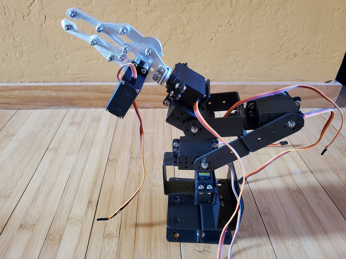
An end effector is the component on a robot arm that has an effect on the environment. For example, consider this robotic arm below. The end effector is the silver robotic gripper.
An end effector could also be a robotic hand or a vacuum gripper.
A joint on a robot is like a joint on the human body (shoulder, elbow, et.). A joint is the moveable part of a robot.
For a typical robotic arm, a joint is a motor that connects one link to another link. To continue the analogy of the human body, the lower arm and upper arm links are connected by the elbow joint.
In the photo of the robotic arm above, there are 6 joints (i.e. 6 motors). Going from the base of the robot to the gripper, you have a:
Base joint (Motor 0)
Shoulder joint (Motor 1)
Elbow joint (Motor 2)
Wrist joint (Motor 3)
Hand joint (Motor 4)
Gripper Joint (i.e. the silver claw) (Motor 5)
Links (i.e. the black brackets in the robotic arm above) are the stiff components that connect the joints (i.e. servo motors) together.