

In this post I will discuss Occam’s razor and how it relates to machine learning.
What is Occam’s Razor?
Occam’s razor argues that the simplest explanation is the one most likely to be correct.
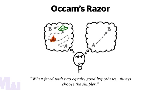
Image Source: ClubStreetPost.com
How is Occam’s Razor Relevant in Machine Learning?
Occam’s Razor is one of the principles that guides us when we are trying to select the appropriate model for a particular machine learning problem. If the model is too simple, it will make useless predictions. If the model is too complex (loaded with attributes), it will not generalize well.
Imagine, for example, you are trying to predict a student’s college GPA. A simple model would be one that is based entirely on a student’s SAT score.
College GPA = Θ * (SAT Score)
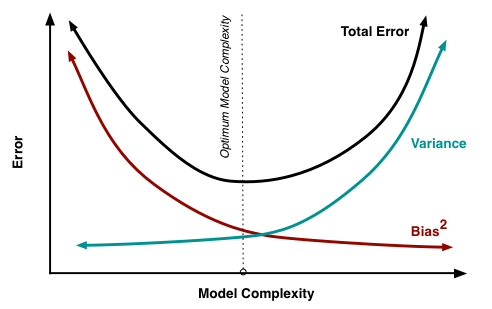
While this model is very simple, it might not be very accurate because often a college student’s GPA is dependent on factors other than just his or her SAT score. It is severely underfit and inflexible. In machine learning jargon, we would say this type of model has high bias, but low variance.
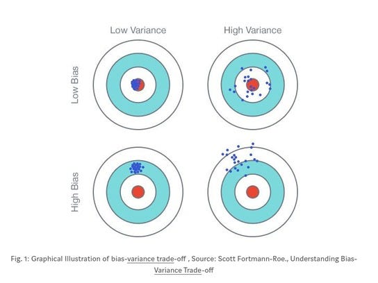
In general, the more inflexible a model, the higher the bias. Also, the noisier the model, the higher the variance. This is known as the bias–variance tradeoff.
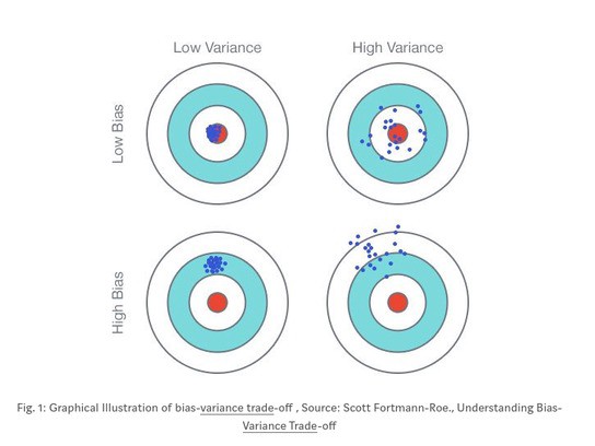
Image Source: Medium.com
If the model is too complex and loaded with attributes, it is at risk of capturing noise in the data that could be due entirely to random chance. It would make amazing predictions on the training data set, but it would perform poorly when faced with a new data set. It won’t generalize well because it is severely overfit. It has high variance and low bias.
A real world example would be like trying to predict a person’s college gpa based on his or her SAT score, high school GPA, middle school GPA, socio-economic status, city of birth, hair color, favorite NBA team, favorite food, and average daily sleep duration.
College GPA = Θ1 * (SAT Score) + Θ2 * High School GPA + Θ3 * Middle School GPA + Θ4 * Socio-Economic status + Θ5 * City of Birth + Θ6 * Hair Color + Θ7 * Favorite NBA Team + Θ8 * Favorite Food + Θ9 * Average Daily Sleep Duration
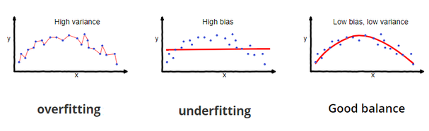
Image Source: Scott Fortman Roe
In machine learning there was always this balance of bias vs. variance, inflexibility vs. flexibility, parsimony vs. prodigality.

How Does Regularization Fit in With All This and the Quest to Solve Overfitting?
Regularization is a technique designed to introduce simplicity to an overly complex model. It is designed to help solve overfitting by working on the assumption that smaller weights are better because they generate less complex models. Regularization does this by adding an additional term (the regularization parameter λ) to the expression that represents the squared difference between the model’s predicted value and the actual value. You can think of this extra term as the “model complexity factor.”
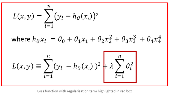
Image Source: Medium.com
λ is a penalty term that “penalizes” the Learner from getting too complex by discouraging large weights that lead to overfit models.
What are the Negative Effects of Regularization?
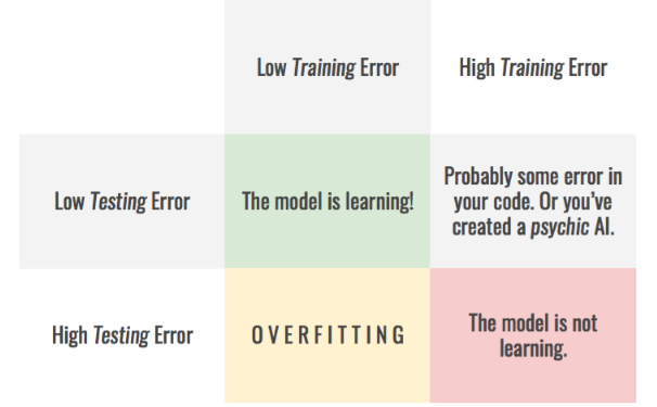
Image Source: Medium.com
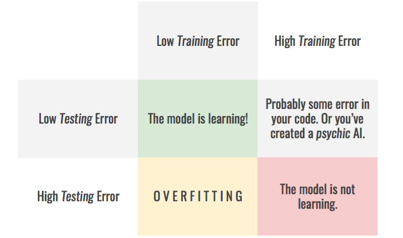
Regularization is designed to solve overfitting. The only negative effect I could think of would be the fact that the selection of the parameter λ is personal. What you chose for λ will be different than what I would choose. It therefore might not be as easy for me to reproduce the results you get, and this might as you stated, possibly influence and bias the model in the opposite direction of the desired result.