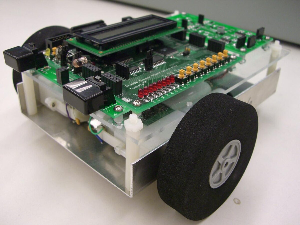
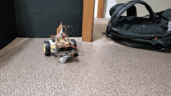
In this tutorial, we will learn how to create a state space model for a mobile robot. Specifically, we’ll take a look at a type of mobile robot called a differential drive robot. A differential drive robot is a robot like the one on the cover photo of this post, as well as this one below. It is called differential drive because each wheel is driven independently from the other. 

Prerequisites

• Basic linear algebra
  • You understand what a matrix and a vector are.
  • You know how to multiply two matrices together.
• You know what a partial derivative is.
• Optional: Python 3.7 or higher (just needed for the last part of this tutorial)

There are a lot of tutorials on YouTube if you don’t have the prerequisites above (e.g. Khan Academy).

What is a State Space Model?

A state space model (often called the state transition model) is a mathematical equation that represents the motion of a robotic system from one timestep to the next. It shows how the current position (e.g. X, Y coordinate) and orientation (yaw (heading) angle γ) of the robot in the world is impacted by changes to the control inputs into the robot (e.g. velocity in meters per second…often represented by the variable v).

Note: In a real-world scenario, we would need to represent the world the robot is in (e.g. a room in your house, etc.) as an x,y,z coordinate grid.

Deriving the Equations

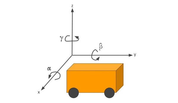
Consider the mobile robot below. It is moving around on the flat x-y coordinate plane.

Let’s look at it from an aerial view.

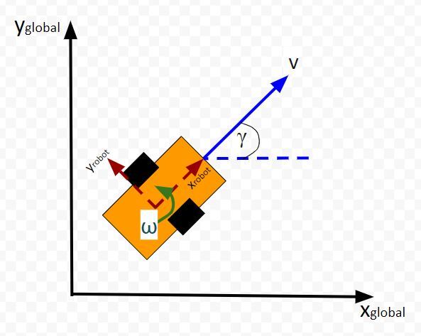
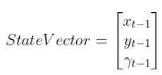
What is the position and orientation of the robot in the world (i.e. global reference frame)? The position and orientation of a robot make up what we call the state vector.

Note that x and y as well as the yaw angle γ are in the global reference frame.

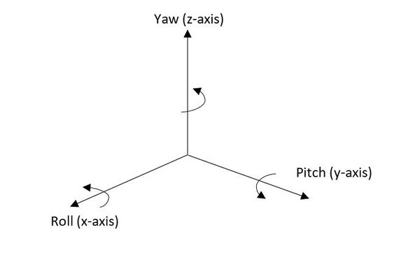
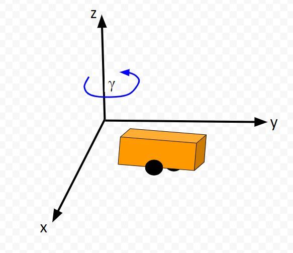
The yaw angle γ describes the rotation around the z-axis (coming out of the page in the image above) in the counterclockwise direction (from the x axis). The units for the yaw angle are typically radians.

ω is the rotation rate (i.e. angular velocity or yaw rate) around the global z axis. Typically the units on this variable is radians per second.

The velocity of the robot v is in terms of the robot reference frame (labeled x_robot and y_robot). 

In terms of the global reference frame we can break v down into two components: 

• velocity in the x direction v_x 
• velocity in the y direction v_y. 

In most of my applications, I express the velocity in meters per second.

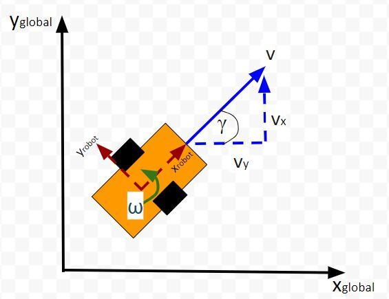
Using trigonometry, we know that:

• cos(γ) = v_x/v 
• sin(γ) = v_x/v 

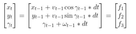
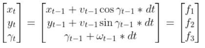
Therefore, with respect to the global reference frame, the robot’s motion equations are as follows:

linear velocity in the x direction = v_x = vcos(γ)

linear velocity in the y direction = v_y = vsin(γ)

angular velocity around the z axis = ω

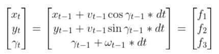
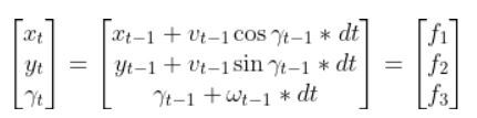
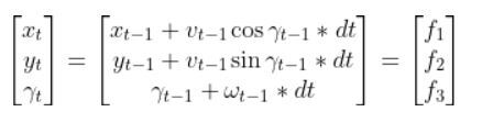
Now let’s suppose at time t-1, the robot has the current state (x position, y position, yaw angle γ):

We move forward one timestep dt. What is the state of the robot at time t? In other words, where is the robot location, and how is the robot oriented? 

Remember that distance = velocity * time. 

Therefore,

Converting the Equations to a State Space Model

We now know how to describe the motion of the robot mathematically. However the equation above is nonlinear. For some applications, like using the Kalman Filter (I’ll cover Kalman Filters in a future post), we need to make our state space equations linear.

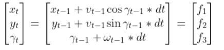
How do we take this equation that is nonlinear (note the cosines and sines)…

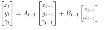
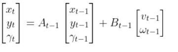
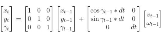
…and convert it into a form that looks like the equation of a line? In mathematical jargon, we want to make the equation above a linear discrete-time state space model of the following form.

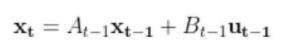
where:

x_t is our entire current state vector [x_t, y_t,γ_t]  (i.e. note x_t in bold is the entire state vector…don’t get that confused with x_t, which is just the x coordinate of the robot at time t)

x_t-1 is the state of the mobile robot at the previous timestep: [x_t-1, y_t-1,γ_t-1]

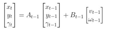
u_t-1 represents the control input vector at the previous timestep [v_t-1, ω_t-1] = [forward velocity, angular velocity]. 

I’ll get to what the A and B matrices represent later in this post.

Let’s write out the full form of the linear state space model equation:

Let’s go through this equation term by term to make sure we understand everything so we can convert this equation below into the form above:

How to Calculate the A Matrix

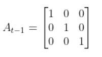
A is a matrix. The number of rows in the A matrix is equal to the number of states, and the number of columns in the A matrix is equal to the number of states. In this mobile robot example, we have three states.

The A matrix expresses how the state of the system [x position,y position,yaw angle γ] changes from t-1 to t when no control command is executed (i.e. when we don’t give any speed (velocity) commands to the robot). 

Typically a robot on wheels only drives when the wheels are commanded to turn. Therefore, for this case, A is the identity matrix (Note that A is sometimes F in the literature).

In other applications, A might not be the identity matrix. An example is a helicopter. The state of a helicopter flying around in the air changes even if you give it no velocity command. Gravity will pull the helicopter downward to Earth regardless of what you do. It will eventually crash if you give it no velocity commands.

Formally, to calculate A, you start with the equation for each state vector variable. In our mobile robot example, that is this stuff below.

Our system is expressed as a nonlinear system now because the state is a function of cosines and sines (which are nonlinear trigonometric operations).

To get our state space model in this form…

…we need to “linearize” the nonlinear equations. To do this, we need to calculate the Jacobian, which is nothing more than a fancy name for “matrix of partial derivatives.” 

Do you remember the equation for a straight line from grade school: y=mx+b? m is the slope. It is “change in y / change in x”.

The Jacobian is nothing more than a multivariable form of the slope m. It is “change in y1/x1, change in y2/x2, change in y3/x3, etc….”  

You can consider the Jacobian a slope on steroids. It represents how fast a group of variables (as opposed to just one variable…(e.g. m = rise/run = change in y/change in x) are changing with respect to another group of variables.

You start with this here:

You then calculate the partial derivative of the state vector at time t with respect to the states at time t-1. Don’t be scared at all the funny symbols inside this matrix A. When you’re calculating the Jacobian matrix, you calculate each partial derivative, one at a time.

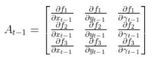
You will have to calculate 9 partial derivatives in total for this example. 

Again, if you are a bit rusty on calculating partial derivatives, there are some good tutorials online. We’ll do an example calculation now so you can see how this works.

Let’s calculate the first partial derivative in the upper left corner of the matrix.

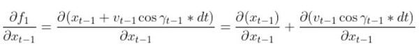
and

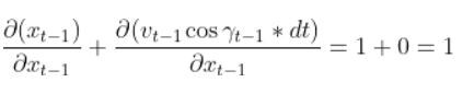
So, 1 goes in the upper-left corner of the matrix.

If you calculate all 9 partial derivatives above, you’ll get:

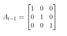
which is the identity matrix.

If you actually calculate these partial derivatives, you will get the following for A_{t-1}:

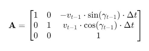
Since we assume 0 for the control inputs, A becomes the identity matrix.

The assumption that the control inputs (v_{t-1} and ω_{t-1}) are zero when calculating the A matrix is based on the physical characteristics of the differential drive mobile robot and the purpose of the A matrix in the state space model.

Physical characteristics of the robot:

A differential drive mobile robot typically only moves when its wheels are commanded to turn. If no control input is given (i.e., the robot is not commanded to move), the robot will remain stationary, and its position and orientation will not change from one time step to the next.

Purpose of the A matrix:

In the state space model, the A matrix is used to express how the state of the system [x position, y position, yaw angle γ] changes from time step t-1 to t when no control command is executed. It represents the natural evolution of the system state without any external influence from the control inputs.

By setting v_{t-1} and ω_{t-1} to zero when calculating the A matrix, we are essentially modeling the behavior of the robot when it is not being actively controlled. This is a valid assumption because we are interested in understanding how the system state evolves on its own, without any control commands.

Linearization at a Specific Point

• Linearizing a nonlinear system involves finding the Jacobian matrix at a specific operating point.
• The chosen operating point here is where the robot is stationary (i.e., no control inputs).

Use Case: Kalman Filtering

The assumption that the A matrix is an identity matrix when no control inputs are given is particularly useful in the context of Kalman filtering for a few reasons:

1. Simplification of the prediction step: In the Kalman filter, the prediction step is responsible for estimating the robot’s state at the next time step based on its current state and the control inputs. By assuming that the A matrix is an identity matrix, the prediction step becomes simpler. The predicted state is essentially the same as the current state if no control inputs are given, which aligns with the physical behavior of the robot.
2. Focus on the effect of control inputs: With the A matrix being an identity matrix, the Kalman filter can focus more on the effect of the control inputs on the robot’s state. The B matrix captures how the control inputs (linear and angular velocities) influence the change in the robot’s position and orientation. This allows the Kalman filter to effectively incorporate the control inputs into the state estimation process. We’ll calculate the B matrix in the next section.
3. Modeling the uncertainty: The Kalman filter is designed to handle uncertainty in the robot’s motion and measurements. By assuming that the A matrix is an identity matrix, the uncertainty in the robot’s motion is primarily attributed to the control inputs and the process noise. The process noise can be modeled to account for factors like wheel slippage, uneven surfaces, or other disturbances that affect the robot’s motion. The Kalman filter uses this uncertainty information to estimate the robot’s state more accurately.
4. Computational efficiency: Using an identity matrix for the A matrix can lead to more efficient computations in the Kalman filter. Since the identity matrix has a simple structure (1s on the diagonal and 0s elsewhere), it can simplify the matrix calculations involved in the prediction and update steps of the filter. This can be beneficial when running the Kalman filter on resource-constrained systems or when real-time performance is critical.

It’s important to note that the assumption of an identity matrix for A is specific to the case when no control inputs are given. In the overall Kalman filter algorithm, the actual control inputs (linear and angular velocities) are still used in the prediction step to estimate the robot’s state at the next time step.

By leveraging this assumption, the Kalman filter can more effectively estimate the robot’s state, account for uncertainty, and incorporate the effect of control inputs, all while maintaining computational efficiency. This makes it a powerful tool for state estimation and localization in mobile robot applications.

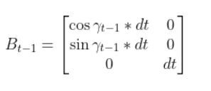
How to Calculate the B Matrix

The B matrix in our running example of a mobile robot is a 3×2 matrix. 

The B matrix has the same number of rows as the number of states and has the same number of columns as the number of control inputs. 

The control inputs in this example are the linear velocity (v) and the angular velocity around the z axis, ω (also known as the “yaw rate”).

The B matrix expresses how the state of the system (i.e. [x,y,γ]) changes from t-1 to t due to the control commands (i.e. control inputs v and ω)

Since we’re dealing with a robotic car here, we know that if we apply forward and angular velocity commands to the car, the car will move.

The equation for B is as follows. We need to calculate yet another Jacobian matrix. However, unlike our calculation for the A matrix, we need to compute the partial derivative of the state vector at time t with respect to the control inputs at time t-1.

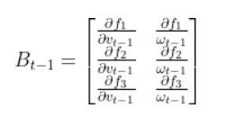
Remember the equations for f₁, f₂, and f₃:

If you calculate the 6 partial derivatives, you’ll get this for the B matrix below:

Putting It All Together

Ok, so how do we get from this:

Into this form:

We now know the A and B matrices, so we can plug those in. The final state space model for our differential drive robot is as follows:

where v_t-1 is the linear velocity of the robot in the robot’s reference frame, and ω_t-1 is the angular velocity in the robot’s reference frame.

And there you have it. If you know the current position of the robot (x,y), the orientation of the robot (yaw angle γ), the linear velocity of the robot, the angular velocity of the robot, and the change in time from one timestep to the next, you can calculate the state of the robot at the next timestep.

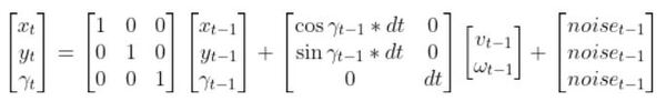
Adding Process Noise

The world isn’t perfect. Sometimes the robot might not act the way you would expect when you want it to execute a specific velocity command. 

It is often common to add a noise term to the state space model to account for randomness in the world. The equation would then be:

Python Code Example for the State Space Model

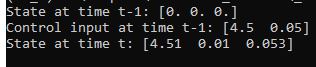
In this section, I’ll show you code in Python for the state space model we have developed in this tutorial. We will assume:

• The robot begins at the origin at a yaw angle of 0 radians. 
• We then apply a forward velocity of 4.5 meters per second at time t-1 and an angular velocity of 0.05 radians per second.

The output will show the state of the robot at the next timestep, time t. I’ll name the file state_space_model.py.

Make sure you have NumPy installed before you run the code. NumPy is a scientific computing library for Python.

If you’re using Anaconda, you can type:

conda install numpy

Alternatively, you can type:

pip install numpy

Here is the code. You can copy and paste this code into your favorite IDE and then run it.

import numpy as np

# Author: Addison Sears-Collins
# https://automaticaddison.com
# Description: A state space model for a differential drive mobile robot

# A matrix
# 3x3 matrix -> number of states x number of states matrix
# Expresses how the state of the system [x,y,yaw] changes 
# from t-1 to t when no control command is executed.
# Typically a robot on wheels only drives when the wheels are commanded
# to turn.
# For this case, A is the identity matrix.
# A is sometimes F in the literature.
A_t_minus_1 = np.array([[1.0,  0,   0],
                        [  0,1.0,   0],
                        [  0,  0, 1.0]])
						
# The estimated state vector at time t-1 in the global 
# reference frame
# [x_t_minus_1, y_t_minus_1, yaw_t_minus_1]
# [meters, meters, radians]
state_estimate_t_minus_1 = np.array([0.0,0.0,0.0])

# The control input vector at time t-1 in the global 
# reference frame
# [v, yaw_rate]
# [meters/second, radians/second]
# In the literature, this is commonly u.
control_vector_t_minus_1 = np.array([4.5, 0.05])

# Noise applied to the forward kinematics (calculation
# of the estimated state at time t from the state
# transition model of the mobile robot). This is a vector
# with the number of elements equal to the number of states
process_noise_v_t_minus_1 = np.array([0.01,0.01,0.003])

yaw_angle = 0.0 # radians
delta_t = 1.0 # seconds

def getB(yaw,dt):
  """
  Calculates and returns the B matrix
  3x2 matix -> number of states x number of control inputs
  The control inputs are the forward speed and the
  rotation rate around the z axis from the x-axis in the 
  counterclockwise direction.
  [v, yaw_rate]
  Expresses how the state of the system [x,y,yaw] changes
  from t-1 to t due to the control commands (i.e. control
  input).
  :param yaw: The yaw (rotation angle around the z axis) in rad 
  :param dt: The change in time from time step t-1 to t in sec
	"""
  B = np.array([[np.cos(yaw)*dt, 0],
                [np.sin(yaw)*dt, 0],
                [0, dt]])
  return B

def main():
  state_estimate_t = A_t_minus_1 @ (
    state_estimate_t_minus_1) + (
    getB(yaw_angle, delta_t)) @ (
    control_vector_t_minus_1) + (
    process_noise_v_t_minus_1)

  print(f'State at time t-1: {state_estimate_t_minus_1}')
  print(f'Control input at time t-1: {control_vector_t_minus_1}')
  print(f'State at time t: {state_estimate_t}') # State after delta_t seconds

main()

Run the code:

python state_space_model.py

Here is the output:

And that’s it for the fundamentals of state space modeling. Once you know the physics of how a robotic system moves from one timestep to the next, you can create a mathematical model in state space form. 

Keep building!