What is Quickprop?

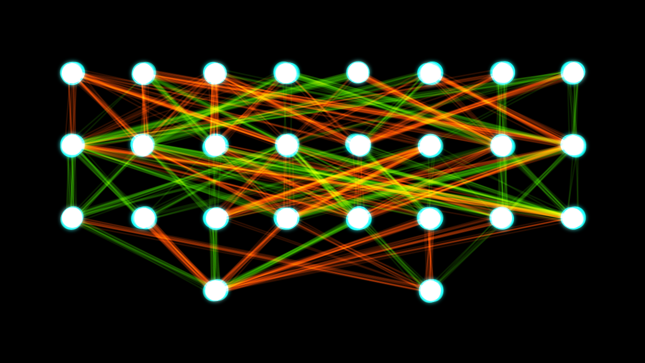
Normal backpropagation when training an artificial feedforward neural network can take a long time to converge on the optimal set of weights. Updating the weights in the first layers of a neural network requires errors that are propagated backwards from the output layer. This procedure might work well for small networks, but when there are a lot of hidden layers, standard backpropagation can really slow down the training process.

Scott E. Fahlman, a Professor Emeritus at Carnegie Mellon University in the School of Computer Science, decided in the late 1980s to speed up backpropagation by inventing a new algorithm called Quickprop which was inspired by Newton’s method, a popular root-finding algorithm.

The idea behind QuickProp is to take the biggest steps possible without overstepping the solution (Kirk, 2015). Instead of the error information propagating backwards from the output layer (as is the case with standard backpropagation), QuickProp needs just the current and previous values of the weights, as well as the error derivative that was calculated during the most recent epoch. This twist on backpropagation means that the weight update process is now entirely local with respect to each node.

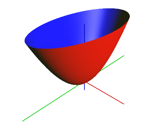
In Quickprop, we assume that the shape of the cost function for a given weight when near its optimal value is a paraboloid. With this assumption we can then follow a method similar to Newton’s method for converging on the optimal solution.

The downside of Quickprop is that it can get chaotic if the surface of the cost function has a lot of local minima (Kirk, 2015).

Title Image Source: Wikimedia Commons

What is the Vanishing Gradient Problem?

The vanishing gradient problem is as follows: As a neural network contains more and more layers, the gradients of the cost function with respect to the weights at each of the nodes gets smaller and smaller, approaching zero. Teeny tiny gradients make the network increasingly more difficult to train.

The vanishing gradient problem is caused by the nature of backpropagation as well as the activation function (e.g. logistic sigmoid function). Backpropagation computes gradients using the chain rule. And since the sigmoid function generates gradients in the range (0, 1), at each step of training, you are multiplying a chain of small numbers together in order to calculate the gradients.

Consistently multiplying smaller and smaller gradient values produces smaller and smaller weight update values since the magnitude of the weight updates (i.e. step size) is proportional to the learning rate and the gradients.

Thus, because the gradients become vanishingly small, the algorithm takes longer and longer to converge on an optimal set of weights. And since the weights will only make teeny tiny changes during each step of the training phase, the weights do not update effectively, and the neural network network losses accuracy.

What is Cascade Correlation?

Cascade correlation is a method that addresses the question of how many hidden layers and how many hidden nodes we need. Instead of starting with a fixed network with a set number of hidden layers and nodes per hidden layer, the cascade correlation method starts with a minimal network and then trains and adds one hidden layer at a time.

How Does Quickprop Address the Vanishing Gradient Problem in Cascade Correlation?

Some scientists have combined the Cascade correlation learning architecture with the Quickprop weight update rule (Abrahart, 2004). When combined in this fashion, Cascade correlation prevents there from being a vanishing gradient problem due to the fact the gradient is never actually propagated from output all the way back to input through the various layers.

As noted by Marquez et al. (2018), “such training of deep networks in a cascade, directly circumvents the well-known vanishing gradient problem by ensuring that the output is always adjacent to the layer being trained.” This is because of the way the weights are locked as new layers are inserted, and the inputs are still tied directly to the outputs.

So to answer the question posed in the title, it’s really the cascade correlation architecture that has the greatest effect on reducing the vanishing gradient problem even though there is some benefit from the Quickprop algorithm.

References

Abrahart, Robert J., Pauline E. Kneale, and Linda M. See. Neural networks for hydrological modelling. Leiden New York: A.A. Balkema Publishers, 2004. Print.

Marquez, Enrique S., Jonathon S. Hare, Mahesan Niranjan: Deep Cascade Learning. IEEE Trans. Neural Netw. Learning Syst. 29(11): 5475-5485 (2018).

Kirk, Matthew, et al. Thoughtful Machine learning : A Test-driven Approach. Sebastopol, California: O’Reilly, 2015. Print.