In this post, I will walk you through the k-means clustering algorithm, step-by-step. We will develop the code for the algorithm from scratch using Python. We will then run the algorithm on a real-world data set, the iris data set (flower classification) from the UCI Machine Learning Repository. Without further ado, let’s get started!
Table of Contents
- What is the K-means Clustering Algorithm?
- K-means Clustering Algorithm Design
- K-means Clustering Algorithm in Python, Coded From Scratch
- Output Statistics of K-means Clustering on the Iris Data Set
What is the K-means Clustering Algorithm?
The K-means algorithm is an unsupervised clustering algorithm (the target variable we want to predict is not available) that is used to group unlabeled data set instances into clusters based on similar attributes.
Step 1: Choose a Value for K and Select the Initial Centroids
The first step of K-means is to determine the valve for k, the number of clusters you want to group your data set into. We then randomly select k cluster centroids (i.e. k random instances) from the data set, where k is some positive integer.
Step 2: Cluster Assignment
The next step is the cluster assignment step. This step involves going through each of the instances and assigning that instance to the cluster centroid closest to it.
Step 3: Move Centroid
The next part is the move centroid step. We move each of the k centroids to the average of all the instances that were assigned to that cluster centroid.
Step 4: Repeat Steps 2 and 3 Until Centroids Stop Changing
We keep running the cluster assignment and move centroid steps until the cluster centroids stop changing. At that point, the data is deemed clustered.
Andrew Ng, a professor of machine learning at Stanford University, does a good job of showing you visually how k-means clustering works:
K-means Clustering Algorithm Design
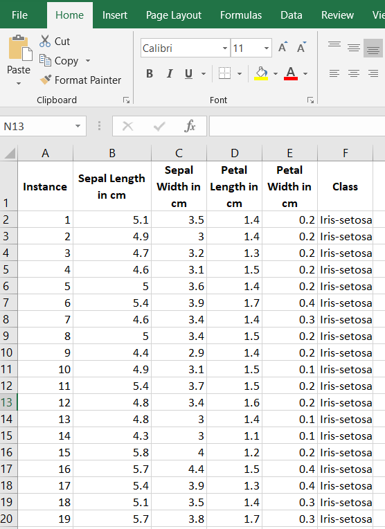
The first thing we need to do is preprocess the iris data set so that it meets the input requirements of both algorithms. Below is the required data format. I downloaded the data into Microsoft Excel and then made sure I had the following columns:
Columns (0 through N)
- 0: Instance ID
- 1: Attribute 1
- 2: Attribute 2
- 3: Attribute 3
- …
- N: Actual Class (used for classification accuracy calculation)
The program then adds 4 additional columns.
- N + 1: Cluster
- N + 2: Silhouette Coefficient
- N + 3: Predicted Class
- N + 4: Prediction Correct? (1 if yes, 0 if no)
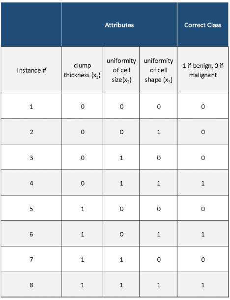
Here is what your data set should look like:
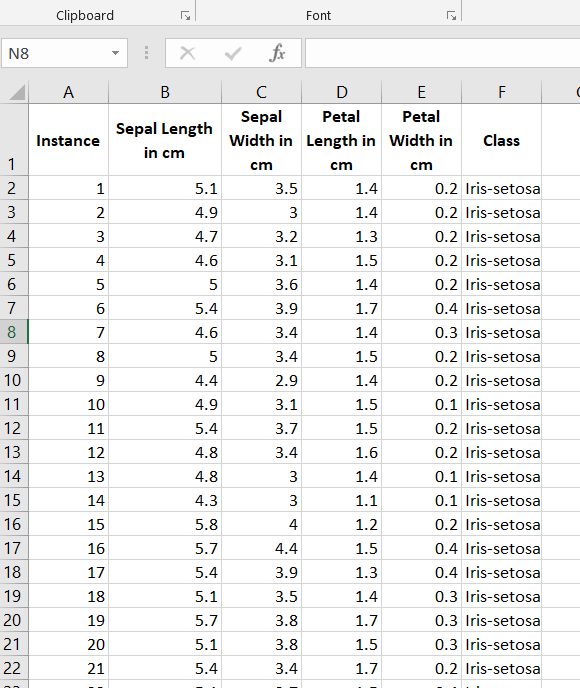
The iris data set contains 3 classes of 50 instances each (150 instances in total), where each class refers to a different type of iris flower. There are 4 attributes in the data set.
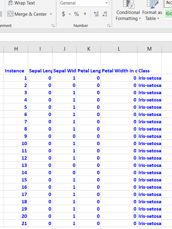
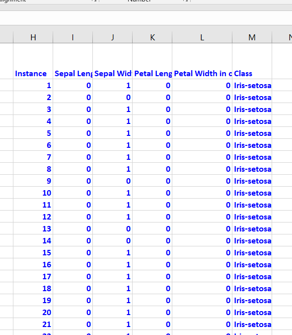
Binarization is optional, but I prefer to do it since it speeds up the attribute selection process. You need to go through each attribute, one by one. Attribute values greater than the mean of the attribute need to be changed to 1, otherwise set it to 0. Here is the general Excel formula:
=IF(B2>AVERAGE(B$2:B$151),1,0)
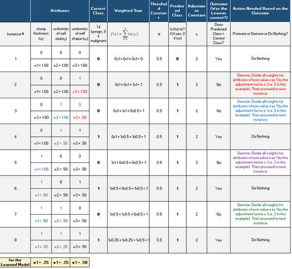
Here is how the data looks after the binarization:
Save the file as a csv file (comma-delimited), and load it into the program below (Python).
Here is a link to the final data set I used.
K-means Clustering Algorithm in Python, Coded From Scratch
K-means appears to be particularly sensitive to the starting centroids. The starting centroids for the k clusters were chosen at random. When these centroids started out poor, the algorithm took longer to converge to a solution. Future work would be to fine-tune the initial centroid selection process.
Here is the full code for k-means clustering. Don’t be scared at how long this code is. I include a bunch of comments at each step so that you know what is going on. Just copy and paste this into your favorite IDE and run it!
import pandas as pd # Import Pandas library
import numpy as np # Import Numpy library

# File name: kmeans.py
# Author: Addison Sears-Collins
# Date created: 6/12/2019
# Python version: 3.7
# Description: Implementation of K-means clustering algorithm from scratch.
# K-means algorithm is a clustering algorithm that is used to group
# unlabeled data set instances into clusters based on similar attributes.

# Required Data Set Format:
# Columns (0 through N)
# 0: Instance ID
# 1: Attribute 1
# 2: Attribute 2
# 3: Attribute 3
# ...
# N: Actual Class (used for classification accuracy calculation)

# This program then adds 4 additional columns.
# N + 1: Cluster
# N + 2: Silhouette Coefficient
# N + 3: Predicted Class
# N + 4: Prediction Correct? (1 if yes, 0 if no)

################ INPUT YOUR OWN VALUES IN THIS SECTION ######################
ALGORITHM_NAME = "K-means"
DATA_PATH = "iris_dataset.txt"  # Directory where data set is located
TEST_STATS_FILE = "iris_dataset_kmeans_test_stats.txt"#Testing statistics
TEST_OUT_FILE = "iris_dataset_kmeans_test_out.txt" # Testing output
# Show functioning of the program
TRACE_RUNS_FILE  = "iris_dataset_kmeans_trace_runs.txt"
SEPARATOR = ","  # Separator for the data set (e.g. "\t" for tab data)
#############################################################################

# Open a new file to save trace runs
outfile3 = open(TRACE_RUNS_FILE,"w")

# Read the full text file and store records in a Pandas dataframe
pd_full_data_set = pd.read_csv(DATA_PATH, sep=SEPARATOR)

# Copy the dataframe into a new dataframe so we don't mess up the
# original data
pd_data_set = pd_full_data_set.copy()

# Calculate the number of instances, columns, and attributes in the
# training data set. Assumes 1 column for the instance ID and 1 column
# for the class. Record the index of the column that contains
# the actual class
no_of_instances = len(pd_data_set.index) # number of rows
no_of_columns = len(pd_data_set.columns) # number of columns
no_of_attributes = no_of_columns - 2
actual_class_column = no_of_columns - 1

# Store class values in a column and then create a list of unique
# classes and store in a dataframe and a Numpy array
unique_class_list_df = pd_data_set.iloc[:,actual_class_column]
unique_class_list_np = unique_class_list_df.unique() #Numpy array
unique_class_list_df = unique_class_list_df.drop_duplicates()#Pandas df

# Record the number of unique classes in the data set
num_unique_classes = len(unique_class_list_df)

# Record the value for K, the number of clusters
K = num_unique_classes

# Remove the Instance and the Actual Class Column to create an unlabled
# data set
instance_id_colname = pd_data_set.columns[0]
class_column_colname = pd_data_set.columns[actual_class_column]
pd_data_set = pd_data_set.drop(columns = [ # Each row is a different instance
        instance_id_colname, class_column_colname])

# Convert dataframe into a Numpy array
np_data_set = pd_data_set.to_numpy(copy=True)

# Randomly select k instances from the data set.
# These will be the cluster centroids for the first iteration
# of the algorithm.
centroids = np_data_set[np.random.choice(np_data_set.shape[
    0], size=K, replace=False), :]


##################### Cluster Assignment Step ################################
# Go through each instance and assign that instance to the closest
# centroid (based on Euclidean distance).

# Initialize an array which will contain the cluster assignments for each
# instance.
cluster_assignments = np.empty(no_of_instances)

# Goes True if new centroids are the same as the old centroids
centroids_the_same = False

# Sets the maximum number of iterations
max_iterations = 300

while max_iterations > 0 and not(centroids_the_same):
    # Go through each data point and assign it to the nearest centroid
    for row in range(0, no_of_instances):

        this_instance = np_data_set[row]

        # Calculate the Euclidean distance of each instance in the data set
        # from each of the centroids
        # Find the centroid with the minimum distance and assign the instance
        # to that centroid.
        # Record that centroid in the cluster assignments array.

        # Reset the minimum distance to infinity
        min_distance = float("inf")

        for row_centroid in range(0, K):
            this_centroid = centroids[row_centroid]

            # Calculate the Euclidean distance from this instance to the
            # centroid
            distance = np.linalg.norm(this_instance - this_centroid)

            # If we have a centroid that is closer to this instance,
            # update the cluster assignment for this instance.
            if distance < min_distance:
                cluster_assignments[row] = row_centroid
                min_distance = distance # Update the minimum distance

    # Print after each cluster assignment has completed
    print("Cluster assignments completed for all " + str(
        no_of_instances) + " instances. Here they are:")
    print(cluster_assignments)
    print()
    print("Now calculating the new centroids...")
    print()

    outfile3.write("Cluster assignments completed for all " + str(
        no_of_instances) + " instances. Here they are:"+ "\n")
    outfile3.write(str(cluster_assignments))
    outfile3.write("\n")
    outfile3.write("\n")
    outfile3.write("Now calculating the new centroids..." + "\n")
    outfile3.write("\n")


    ##################### Move Centroid Step ################################
    # Calculate the centroids of the clusters by computing the average
    # of the attribute values of the instances in each cluster
    # For each row in the centroids 2D array

    # Store the old centroids
    old_centroids = centroids.copy()

    for row_centroid in range(0, K):

        # For each column of each row of the centroids 2D array
        for col_centroid in range(0, no_of_attributes):

            # Reset the running sum and the counter
            running_sum = 0.0
            count = 0.0
            average = None

            for row in range(0, no_of_instances):

                # If this instance belongs to this cluster
                if(row_centroid == cluster_assignments[row]):

                    # Add this value to the running sum
                    running_sum += np_data_set[row,col_centroid]

                    # Increment the counter
                    count += 1

                    if (count > 0):
                        # Calculate the average
                        average = running_sum / count

            # Update the centroids array with this average
            centroids[row_centroid,col_centroid] = average

    # Print to after each cluster assignment has completed
    print("New centroids have been created. Here they are:")
    print(centroids)
    print()

    outfile3.write("New centroids have been created. Here they are:" + "\n")
    outfile3.write(str(centroids))
    outfile3.write("\n")
    outfile3.write("\n")

    # Check if cluster centroids are the same
    centroids_the_same = np.array_equal(old_centroids,centroids)

    if centroids_the_same:
        print(
        "Cluster membership is unchanged. Stopping criteria has been met.")
        outfile3.write("Cluster membership is unchanged. ")
        outfile3.write("Stopping criteria has been met." + "\n")
        outfile3.write("\n")

    # Update the number of iterations
    max_iterations -= 1

# Record the actual class column name
actual_class_col_name = pd_full_data_set.columns[len(
    pd_full_data_set.columns) - 1]

# Add 4 additional columns to the original data frame
pd_full_data_set = pd_full_data_set.reindex(
      columns=[*pd_full_data_set.columns.tolist(
      ), 'Cluster', 'Silhouette Coefficient', 'Predicted Class', (
      'Prediction Correct?')])

# Add the final cluster assignments to the Pandas dataframe
pd_full_data_set['Cluster'] = cluster_assignments

outfile3.write("Calculating the Silhouette Coefficients. Please wait..." + "\n")
outfile3.write("\n")
print()
print("Calculating the Silhouette Coefficients. Please wait...")
print()
################## Calculate the Silhouette Coefficients ######################
# Rewards clusterings that have good cohesion and good separation. Varies
# between 1 and -1. -1 means bad clustering, 1 means great clustering.

# 1. For each instance calculate the average distance to all other instances
# in that cluster. This is a.
# 2. (Find the average distance to all the instances in the nearest neighbor
# cluster). For each instance and any cluster that does not contain the
# instance calculate the average distance to all
# of the points in that other cluster. Then return the minimum such value
# over all of the clusters. This is b.
# 3. For each instance calculate the Silhouette Coefficient s where
# s = (b-a)/max(a,b)
# Store the value in the data frame

silhouette_column = actual_class_column + 2

# Go through one instance at a time
for row in range(0, no_of_instances):

    this_instance = np_data_set[row]
    this_cluster = cluster_assignments[row]

    a = None
    running_sum = 0.0
    counter = 0.0

    # Calculate the average distance to all other instances
    # in this cluster. This is a.
    # Go through one instance at a time
    for row_2 in range(0, no_of_instances):

        # If the other instance is in the same cluster as this instance
        if this_cluster == cluster_assignments[row_2]:

            # Calculate the distance
            distance = np.linalg.norm(this_instance - np_data_set[row_2])

            # Add the distance to the running sum
            running_sum += distance
            counter += 1

    # Calculate the value for a
    if counter > 0:
        a = running_sum / counter

    # For each instance and any cluster that does not contain the
    # instance calculate the average distance to all
    # of the points in that other cluster. Then return the minimum such value
    # over all of the clusters. This is b.
    b = float("inf")

    for clstr in range(0, K):

        running_sum = 0.0
        counter = 0.0

        # Must be other clusters, not the one this instance is in
        if clstr != this_cluster:

            # Calculate the average distance to instances in that
            # other cluster
            for row_3 in range(0, no_of_instances):

                if cluster_assignments[row_3] == clstr:

                    # Calculate the distance
                    distance = np.linalg.norm(this_instance - np_data_set[
                        row_3])

                    # Add the distance to the running sum
                    running_sum += distance
                    counter += 1

            if counter > 0:
                avg_distance_to_cluster = running_sum / counter

            # Update b if we have a new minimum
            if avg_distance_to_cluster < b:
                b = avg_distance_to_cluster

    # Calculate the Silhouette Coefficient s where s = (b-a)/max(a,b)
    s = (b - a) / max(a,b)

    # Store the Silhouette Coefficient in the Pandas data frame
    pd_full_data_set.iloc[row,silhouette_column] = s

#################### Predict the Class #######################################
# For each cluster, determine the predominant class and assign that
# class to the cluster. Then determine if the prediction was correct.
# Create a data frame that maps clusters to actual classes
class_mappings = pd.DataFrame(index=range(K),columns=range(1))

for clstr in range(0, K):

    # Select rows whose column equals that cluster value
    temp_df = pd_full_data_set.loc[pd_full_data_set['Cluster'] == clstr]

    # Select the predominant class
    class_mappings.iloc[clstr,0] = temp_df.mode()[actual_class_col_name][0]

cluster_column = actual_class_column + 1
pred_class_column = actual_class_column + 3
pred_correct_column = actual_class_column + 4

# Assign the relevant class to each instance
# See if prediction was correct
for row in range(0, no_of_instances):

    # Go through each of the clusters to check if the instance is a member
    # of that cluster
    for clstr in range(0, K):
        if clstr == pd_full_data_set.iloc[row,cluster_column]:

            # Assign the relevant class to this instance
            pd_full_data_set.iloc[
                row,pred_class_column] = class_mappings.iloc[clstr,0]

    # If the prediction was correct
    if pd_full_data_set.iloc[row,pred_class_column] == pd_full_data_set.iloc[
        row,actual_class_column]:
        pd_full_data_set.iloc[row,pred_correct_column] = 1
    else: # If incorrect prediction
        pd_full_data_set.iloc[row,pred_correct_column] = 0

# Write dataframe to a file
pd_full_data_set.to_csv(TEST_OUT_FILE, sep=",", header=True)

# Print data frame to the console
print()
print()
print("Data Set")
print(pd_full_data_set)
print()
print()

################### Summary Statistics #######################################
# Calculate the average Silhouette Coefficient for the data set
# Calculate the accuracy of the clustering-based classifier

# Open a new file to save the summary statistics
outfile1 = open(TEST_STATS_FILE,"w")

# Write to a file
outfile1.write("----------------------------------------------------------\n")
outfile1.write(ALGORITHM_NAME + " Summary Statistics (Testing)\n")
outfile1.write("----------------------------------------------------------\n")
outfile1.write("Data Set : " + DATA_PATH + "\n")

# Write the relevant stats to a file
outfile1.write("\n")
outfile1.write("Number of Instances : " + str(no_of_instances) + "\n")
outfile1.write("\n")
outfile1.write("Value for k : " + str(K) + "\n")

# Calculate average Silhouette Coefficient for the data set
silhouette_coefficient = pd_full_data_set.loc[
    :,"Silhouette Coefficient"].mean()

# Write the Silhouette Coefficient to the file
outfile1.write("Silhouette Coefficient : " + str(
    silhouette_coefficient) + "\n")

# accuracy = (total correct predictions)/(total number of predictions)
accuracy = (pd_full_data_set.iloc[
        :,pred_correct_column].sum())/no_of_instances

accuracy *= 100

# Write accuracy to the file
outfile1.write("Accuracy : " + str(accuracy) + "%\n")

# Print statistics to console
print()
print()
print("-------------------------------------------------------")
print(ALGORITHM_NAME + " Summary Statistics (Testing)")
print("-------------------------------------------------------")
print("Data Set : " + DATA_PATH)

# Print the relevant stats to the console
print()
print("Number of Instances : " + str(no_of_instances))
print("Value for k : " + str(K))

# Print the Silhouette Coefficient to the console
print("Silhouette Coefficient : " + str(
    silhouette_coefficient))

# Print accuracy to the console
print("Accuracy : " + str(accuracy) + "%")

# Close the files
outfile1.close()
outfile3.close()
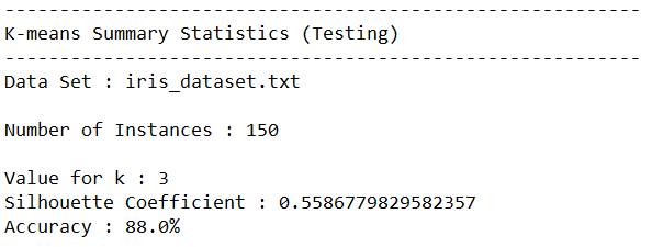
Output Statistics of K-means Clustering on the Iris Data Set
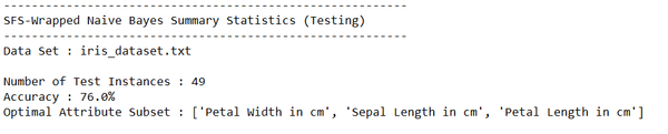
This section shows the results for the runs of K-means Clustering on the iris data set.
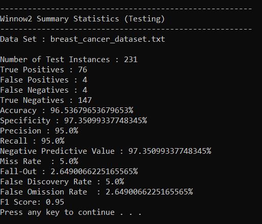
Test Statistics
Trace Runs
Here are the trace runs of the algorithm.
Output
Here is the output of the algorithm.