In this post, I will walk you through the Stepwise Forward Selection algorithm, step-by-step. We will develop the code for the algorithm from scratch using Python and use it for feature selection for the Naive Bayes algorithm we previously developed. We will then run the algorithm on a real-world data set, the iris data set (flower classification) from the UCI Machine Learning Repository. Without further ado, let’s get started!
Table of Contents
- What is the Stepwise Forward Selection Algorithm?
- Stepwise Forward Selection Implementation
- Stepwise Forward Selection Algorithm in Python, Coded From Scratch
- Output Statistics of Stepwise Forward Selection on the Iris Data Set
What is the Stepwise Forward Selection Algorithm?
One of the fundamental ideas in machine learning is the Curse of Dimensionality – as the number of attributes in the training set grows, you need exponentially more instances to learn the underlying concept. And the more instances you have, the more computational time is required to process the data.
In other words, adding attributes improves performance, to a point. Beyond that point, you need to have exponentially more instances in order for performance to improve. This phenomenon is commonly known as the Hughes Effect (or Hughes Phenomenon).
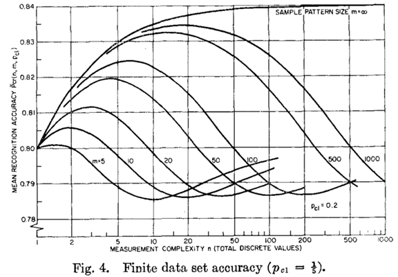
Image Source: Hughes, G. (1968). On the Mean Accuracy Of Statistical Pattern Recognizers. IEEE Transactions on Information Theory, 14(1), 55-63.
In the above image, n = number of attributes and m = number of instances.
One technique for combatting the Curse of Dimensionality is known as Stepwise Forward Selection (SFS). SFS involves selecting only the most relevant attributes for learning and discarding the rest. The metric that determines what attribute is “most relevant” is determined by the programmer. In this project, I will use the classification accuracy of Naïve Bayes.
Because SFS is just a method to create an optimal attribute subset, it needs to be wrapped with another algorithm (in this case Naïve Bayes) that does the actual learning. For this reason, SFS is known as a wrapper method.
The goal of SFS is to reduce the number of features that a machine learning algorithm needs to examine by eliminating unnecessary features and finding an optimal attribute subset.
Suppose we have attributes A1 through Ak which are used to describe a data set D.
A = <A1,…Ak>
SFS begins with an empty attribute set:
A0 = <>
It then selects an attribute from A, one at a time, until the performance (e.g. as measured by classification accuracy) of the target learning algorithm (e.g. Naïve Bayes) on a subset of the training data fails to improve performance.
Stepwise Forward Selection Implementation
The first thing we need to do is preprocess the iris data set so that it meets the input requirements of both algorithms. Below is the required data format. I downloaded the data into Microsoft Excel and then made sure I had the following columns:
Columns (0 through N)
- 0: Instance ID
- 1: Attribute 1
- 2: Attribute 2
- 3: Attribute 3
- …
- N: Actual Class
The program I developed (code is below) then adds 2 additional columns for the testing set.
- N + 1: Predicted Class
- N + 2: Prediction Correct? (1 if yes, 0 if no)
Here is what your data set should look like:
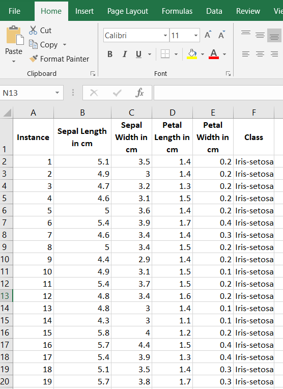
The iris data set contains 3 classes of 50 instances each (150 instances in total), where each class refers to a different type of iris flower. There are 4 attributes in the data set. Here is what an iris flower looks like in case you are interested:

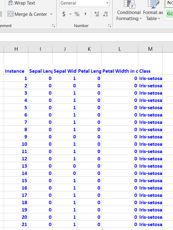
Binarization is optional, but I prefer to do it since it speeds up the attribute selection process. You need to go through each attribute, one by one. Attribute values greater than the mean of the attribute need to be changed to 1, otherwise set it to 0. Here is the general Excel formula:
=IF(B2>AVERAGE(B$2:B$151),1,0)
Here is how the data looks after the binarization:
Save the file as a csv file (comma-delimited), and load it into the program below (Python).
Here is a link to the final data set I used.
Stepwise Forward Selection Algorithm in Python, Coded From Scratch
Naïve Bayes was wrapped with SFS for feature selection. Classification accuracy was used to select the optimal attribute at each step. Once the optimal attribute subset was obtained, Naïve Bayes was run on the complete training set (67% of instances) and testing set (33% of instances), and classification accuracy was calculated.
Here is the code. Just copy and paste it into your favorite IDE. Don’t be scared at how long the code is. I use a lot of comments so that you know what is going on at each step:
import pandas as pd # Import Pandas library
import numpy as np # Import Numpy library

# File name: sfs_naive_bayes.py
# Author: Addison Sears-Collins
# Date created: 6/10/2019
# Python version: 3.7
# Description: Implementation of Naive Bayes which uses Stepwise Forward
# Selection (SFS) for feature selection. This code works for multi-class
# classification problems (e.g. democrat/republican/independent)
# Calculate P(E1|CL0)P(E2|CL0)P(E3|CL0)...P(E#|CL0) * P(CL0) and
# P(E1|CL1)P(E2|CL1)P(E3|CL1)...P(E#|CL1) * P(CL1) and
# P(E1|CL2)P(E2|CL2)P(E3|CL2)...P(E#|CL2) * P(CL2), etc. and predict the
# class with the maximum result.
# E is an attribute, and CL means class.
# Only need class prior probability and likelihoods to make a prediction
# (i.e. the numerator of Bayes formula) since denominators are same for both
# the P(CL0|E1,E2,E3...)*P(CL0) and P(CL1|E1,E2,E3...)*P(CL1), etc. cases
# where P means "probability of" and | means "given".

# Required Data Set Format:
# Columns (0 through N)
# 0: Instance ID
# 1: Attribute 1
# 2: Attribute 2
# 3: Attribute 3
# ...
# N: Actual Class

# This program then adds 2 additional columns for the testing set.
# N + 1: Predicted Class
# N + 2: Prediction Correct? (1 if yes, 0 if no)

################ INPUT YOUR OWN VALUES IN THIS SECTION ######################
ALGORITHM_NAME = "SFS-Wrapped Naive Bayes"
DATA_PATH = "iris_dataset.txt"  # Directory where data set is located
TEST_STATS_FILE = "iris_dataset_naive_bayes_test_stats.txt"#Testing statistics
TEST_OUT_FILE = "iris_dataset_naive_bayes_test_out.txt" # Testing output
# Show functioning of the program
TRACE_RUNS_FILE  = "iris_dataset_naive_bayes_trace_runs.txt"
SEPARATOR = ","  # Separator for the data set (e.g. "\t" for tab data)
TRAINING_DATA_PRCT = 0.67 # % of data set used for training. Default 0.67
testing_data_prct = 1 - TRAINING_DATA_PRCT # % of data set used for testing
SEED = 99  # SEED for the random number generator. Default: 99
#############################################################################

# Open a new file to save trace runs
outfile3 = open(TRACE_RUNS_FILE,"w")

# Naive Bayes algorithm. Accepts a Pandas dataframeas its parameter
def naive_bayes(pd_data):
    # Create a training dataframe by sampling random instances from original data.
    # random_state guarantees that the pseudo-random number generator generates
    # the same sequence of random numbers each time.
    pd_training_data = pd_data.sample(frac=TRAINING_DATA_PRCT, random_state=SEED)

    # Create a testing dataframe. Dropping the training data from the original
    # dataframe ensures training and testing dataframes have different instances
    pd_testing_data = pd_data.drop(pd_training_data.index)

    ######COMMENT OUT THESE TWO LINES BEFORE RUNNING ################
    #pd_training_data = pd_data.iloc[:20] # Used for testing only, gets 1st 20 rows
    #pd_testing_data = pd_data.iloc[20:22,:] # Used for testing only, rows 20 & 21

    # Calculate the number of instances, columns, and attributes in the
    # training data set. Assumes 1 column for the instance ID and 1 column
    # for the class. Record the index of the column that contains
    # the actual class
    no_of_instances_train = len(pd_training_data.index) # number of rows
    no_of_columns_train = len(pd_training_data.columns) # number of columns
    no_of_attributes = no_of_columns_train - 2
    actual_class_column = no_of_columns_train - 1

    # Store class values in a column, sort them, then create a list of unique
    # classes and store in a dataframe and a Numpy array
    unique_class_list_df = pd_training_data.iloc[:,actual_class_column]
    unique_class_list_df = unique_class_list_df.sort_values()
    unique_class_list_np = unique_class_list_df.unique() #Numpy array
    unique_class_list_df = unique_class_list_df.drop_duplicates()#Pandas df

    # Record the number of unique classes in the data set
    num_unique_classes = len(unique_class_list_df)

    # Record the frequency counts of each class in a Numpy array
    freq_cnt_class = pd_training_data.iloc[:,actual_class_column].value_counts(
        sort=True)

    # Record the frequency percentages of each class in a Numpy array
    # This is a list of the class prior probabilities
    class_prior_probs = pd_training_data.iloc[:,actual_class_column].value_counts(
        normalize=True, sort=True)

    # Add 2 additional columns to the testing dataframe
    pd_testing_data = pd_testing_data.reindex(
                      columns=[*pd_testing_data.columns.tolist(
                      ), 'Predicted Class', 'Prediction Correct?'])

    # Calculate the number of instances and columns in the
    # testing data set. Record the index of the column that contains the
    # predicted class and prediction correctness (1 if yes; 0 if no)
    no_of_instances_test = len(pd_testing_data.index) # number of rows
    no_of_columns_test = len(pd_testing_data.columns) # number of columns
    predicted_class_column = no_of_columns_test - 2
    prediction_correct_column = no_of_columns_test - 1

    ######################### Training Phase of the Model ########################
    # Create a an empty dictionary
    my_dict = {}

    # Calculate the likelihood tables for each attribute. If an attribute has
    # four levels, there are (# of unique classes x 4) different probabilities
    # that need to be calculated for that attribute.
    # Start on the first attribute and make your way through all the attributes
    for col in range(1, no_of_attributes + 1):

        # Record the name of this column
        colname = pd_training_data.columns[col]

        # Create a dataframe containing the unique values in the column
        unique_attribute_values_df = pd_training_data[colname].drop_duplicates()
        # Create a Numpy array containing the unique values in the column
        unique_attribute_values_np = pd_training_data[colname].unique()

        # Calculate likelihood of the attribute given each unique class value
        for class_index in range (0, num_unique_classes):

            # For each unique attribute value, calculate the likelihoods
            # for each class
            for attr_val in range (0, unique_attribute_values_np.size) :
                running_sum = 0

                # Calculate N(unique attribute value && class value)
                # Where N means "number of" and && means "and"
                # Go through each row of the training set
                for row in range(0, no_of_instances_train):
                    if (pd_training_data.iloc[row,col] == (
                        unique_attribute_values_df.iloc[attr_val])) and (
                        pd_training_data.iloc[row, actual_class_column] == (
                        unique_class_list_df.iloc[class_index])):
                            running_sum += 1

                # With N(unique attribute value && class value) as the numerator
                # we now need to divide by the total number of times the class
                # appeared in the data set
                try:
                    denominator = freq_cnt_class[class_index]
                except:
                    denominator = 1.0

                likelihood = running_sum / denominator

                # Add a new likelihood to the dictionary
                # Format of search key is
                # <attribute_name><attribute_value><class_value>
                search_key = str(colname) + str(unique_attribute_values_df.iloc[
                             attr_val]) + str(unique_class_list_df.iloc[
                             class_index])
                my_dict[search_key] = likelihood

    # Print the likelihood table to the console
    # print(pd.DataFrame.from_dict(my_dict, orient='index'))

    ################# End of Training Phase of the Naive Bayes Model ########

    ################# Testing Phase of the Naive Bayes Model ################

    # Proceed one instance at a time and calculate the prediction
    for row in range(0, no_of_instances_test):

        # Initialize the prediction outcome
        predicted_class = unique_class_list_df.iloc[0]
        max_numerator_of_bayes = 0.0

        # Calculate the Bayes equation numerator for each test instance
        # That is: P(E1|CL0)P(E2|CL0)P(E3|CL0)...P(E#|CL0) * P(CL0),
        # P(E1|CL1)P(E2|CL1)P(E3|CL1)...P(E#|CL1) * P(CL1)...
        for class_index in range (0, num_unique_classes):

            # Reset the running product with the class
            # prior probability, P(CL)
            try:
                running_product = class_prior_probs[class_index]
            except:
                running_product = 0.0000001 # Class not found in data set

            # Calculation of P(CL) * P(E1|CL) * P(E2|CL) * P(E3|CL)...
            # Format of search key is
            # <attribute_name><attribute_value><class_value>
            # Record each search key value
            for col in range(1, no_of_attributes + 1):
                attribute_name = pd_testing_data.columns[col]
                attribute_value = pd_testing_data.iloc[row,col]
                class_value = unique_class_list_df.iloc[class_index]

                # Set the search key
                key = str(attribute_name) + str(
                          attribute_value) + str(class_value)

                # Update the running product
                try:
                    running_product *= my_dict[key]
                except:
                    running_product *= 0

            # Record the prediction if we have a new max
            # Bayes numerator
            if running_product > max_numerator_of_bayes:
                max_numerator_of_bayes = running_product
                predicted_class = unique_class_list_df.iloc[
                             class_index] # New predicted class

        # Store the prediction in the dataframe
        pd_testing_data.iloc[row,predicted_class_column] = predicted_class

        # Store if the prediction was correct
        if predicted_class == pd_testing_data.iloc[row,actual_class_column]:
            pd_testing_data.iloc[row,prediction_correct_column] = 1
        else:
            pd_testing_data.iloc[row,prediction_correct_column] = 0

    print("-------------------------------------------------------")
    print("Learned Model Predictions on Testing Data Set")
    print("-------------------------------------------------------")

    # Print the revamped dataframe
    print(pd_testing_data)

    # accuracy = (total correct predictions)/(total number of predictions)
    accuracy = (pd_testing_data.iloc[
        :,prediction_correct_column].sum())/no_of_instances_test
    # Return classification accuracy
    return accuracy
    ####################### End Testing Phase ######################################

# Stepwise forward selection method accepts a Pandas dataframe as a parameter
# and then returns the optimal dataframe from that dataframe.
def sfs(pd_data):

    # Record the name of the column that contains the instance IDs and the class
    instance_id_colname = pd_data.columns[0]
    no_of_columns = len(pd_data.columns) # number of columns
    class_column_index = no_of_columns - 1
    class_column_colname = pd_data.columns[class_column_index]

    # Record the number of available attributes
    no_of_available_attributes = no_of_columns - 2

    # Create a dataframe containing the available attributes by removing
    # the Instance and the Class Column
    available_attributes_df = pd_data.drop(columns = [
        instance_id_colname, class_column_colname])

    # Create an empty optimal attribute dataframe containing only the
    # Instance and the Class Columns
    optimal_attributes_df = pd_data[[instance_id_colname,class_column_colname]]

    # Set the base performance to a really low number
    base_performance = -9999.0

    # Check whether adding a new attribute to the optimal attributes dataframe
    # improves performance
    # While there are still available attributes left
    while no_of_available_attributes > 0:
        # Set the best performance to a low number
        best_performance = -9999.0

        # Initialize the best attribute variable to a placeholder
        best_attribute = "Placeholder"

        # For all attributes in the available attribute data frame
        for col in range(0, len(available_attributes_df.columns)):

            # Record the name of this attribute
            this_attr = available_attributes_df.columns[col]

            # Create a new dataframe with this attribute inserted
            temp_opt_attr_df = optimal_attributes_df.copy()
            temp_opt_attr_df.insert(
                loc=1,column=this_attr,value=(available_attributes_df[this_attr]))

            # Run Naive Bayes on this new dataframe and return the
            # classification accuracy
            current_performance = naive_bayes(temp_opt_attr_df)

            # Find the new attribute that yielded the greatest
            # classification accuracy
            if current_performance > best_performance:
                best_performance = current_performance
                best_attribute = this_attr

        # Did adding another feature lead to improvement?
        if best_performance > base_performance:
            base_performance = best_performance

            # Add the best attribute to the optimal attribute data frame
            optimal_attributes_df.insert(
                loc=1,column=best_attribute,value=(
                available_attributes_df[best_attribute]))

            # Remove the best attribute from the available attribute data frame
            available_attributes_df = available_attributes_df.drop(
                columns = [best_attribute])

            # Print the best attribute to the console
            print()
            print(str(best_attribute) + " added to the optimal attribute subset")
            print()

            # Write to file
            outfile3.write(str(
                best_attribute) + (
                " added to the optimal attribute subset") + "\n")

            # Decrement the number of available attributes by 1
            no_of_available_attributes -= 1

            # Print number of attributes remaining to the console
            print()
            print(str(no_of_available_attributes) + " attributes remaining")
            print()
            print()

            # Write to file
            outfile3.write(str(no_of_available_attributes) + (
                " attributes remaining") + "\n" + "\n")

        else:
            print()
            print("Performance did not improve this round.")
            print("End of Stepwise Forward Selection.")
            print()
            outfile3.write("Performance did not improve this round." + "\n")
            outfile3.write("End of Stepwise Forward Selection." + "\n")
            break

    # Return the optimal attribute set
    return optimal_attributes_df


def main():
    # Read the full text file and store records in a Pandas dataframe
    pd_full_data_set = pd.read_csv(DATA_PATH, sep=SEPARATOR)

    # Used for feature selection of large data sets only
    #pd_full_data_set = pd_full_data_set.sample(frac=0.10, random_state=SEED)

    # Runs SFS on the full data set to find the optimal attribute data frame
    optimal_attribute_set = sfs(pd_full_data_set)

    # Write dataframe to a file
    optimal_attribute_set.to_csv(TEST_OUT_FILE, sep=",", header=True)

    # Open a new file to save the summary statistics
    outfile2 = open(TEST_STATS_FILE,"w")

    # Write to a file
    outfile2.write("----------------------------------------------------------\n")
    outfile2.write(ALGORITHM_NAME + " Summary Statistics (Testing)\n")
    outfile2.write("----------------------------------------------------------\n")
    outfile2.write("Data Set : " + DATA_PATH + "\n")

    # Write the relevant stats to a file
    outfile2.write("\n")
    outfile2.write("Number of Test Instances : " +
        str(round(len(optimal_attribute_set.index) * testing_data_prct)) + "\n")

    # Run Naive Bayes on the optimal attribute set
    accuracy = naive_bayes(optimal_attribute_set)
    accuracy *= 100

    # Write accuracy to the file
    outfile2.write("Accuracy : " + str(accuracy) + "%\n")

    # Print statistics to console
    print()
    print()
    print("-------------------------------------------------------")
    print(ALGORITHM_NAME + " Summary Statistics (Testing)")
    print("-------------------------------------------------------")
    print("Data Set : " + DATA_PATH)

    # Print the relevant stats to the console
    print()
    print("Number of Test Instances : " +
        str(round(len(optimal_attribute_set.index) * testing_data_prct)))

    # Print accuracy to the console
    print()
    print("Accuracy : " + str(accuracy) + "%")
    print()

    # Create a dataframe containing the optimal attributes by removing
    # the Instance and the Class Column
    instance_id_colname = optimal_attribute_set.columns[0]
    no_of_columns = len(optimal_attribute_set.columns) # number of columns
    class_column_index = no_of_columns - 1
    class_column_colname = optimal_attribute_set.columns[class_column_index]
    optimal_attribute_set = optimal_attribute_set.drop(columns = [
        instance_id_colname, class_column_colname])

    # Write a list of the optimal attribute set to a file
    outfile2.write("Optimal Attribute Subset : " + str(list(
        optimal_attribute_set)))

    # Print a list of the optimal attribute set
    print("Optimal Attribute Subset : " + str(list(optimal_attribute_set)))
    print()
    print()

    # Close the files
    outfile2.close()
    outfile3.close()

main() # Call the main function
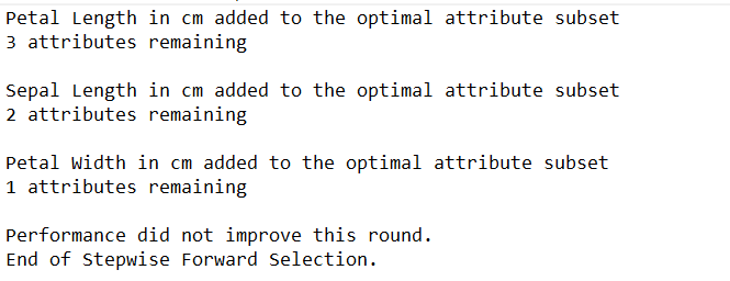
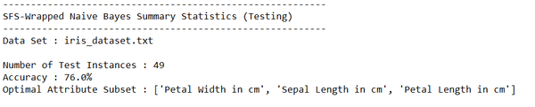
Output Statistics of Stepwise Forward Selection on the Iris Data Set
This section shows the results for the runs of Stepwise Forward Selection wrapped with Naïve Bayes on the iris data set.
Test Statistics
Trace Runs