
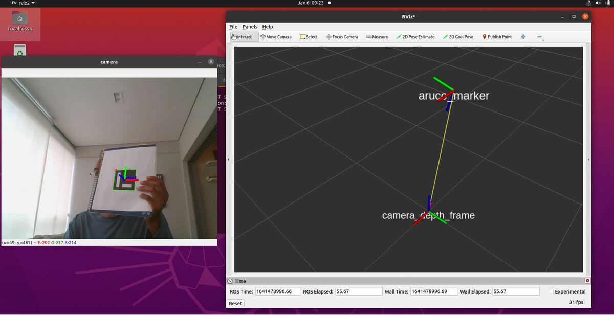
In this tutorial, I will show you how to publish a coordinate transformation between an ArUco marker and a camera (which is usually mounted on the robot). The ArUco marker coordinate frame will be labeled aruco_marker (child frame), and the camera frame will be labeled camera_depth_frame (parent frame).
Here is the output we will achieve:
We will also see how to visualize the coordinate transformation in RViz.
Robotics companies like Boston Dynamics use ArUco markers to precisely connect and recharge at a docking station.
Prerequisites
- ROS 2 Galactic installed on Ubuntu Linux 20.04
- You have already created a ROS 2 workspace. The name of my workspace is dev_ws.
- You have completed this tutorial to make sure OpenCV works with ROS 2 on your computer.
- You have created an ArUco marker.
- You have OpenCV (Python) installed on your system (pip install opencv-contrib-python).
- (Optional) You are able to run the code on this tutorial without any problems.
The link to the opencv_tools package that contains all the full code in this tutorial is here on my Google Drive.
Create the Code
Open a new terminal window, and type:
cd ~/dev_ws/src/opencv_tools/opencv_tools
Open a new Python file named aruco_marker_pose_estimation.py.
gedit aruco_marker_pose_estimation_tf.py
Type the code below into it:
# Publishes a coordinate transformation between an ArUco marker and a camera
# Author:
# - Addison Sears-Collins
# - https://automaticaddison.com
# Import the necessary ROS 2 libraries
import rclpy # Python library for ROS 2
from rclpy.node import Node # Handles the creation of nodes
from cv_bridge import CvBridge # Package to convert between ROS and OpenCV Images
from geometry_msgs.msg import TransformStamped # Handles TransformStamped message
from sensor_msgs.msg import Image # Image is the message type
from tf2_ros import TransformBroadcaster
# Import Python libraries
import cv2 # OpenCV library
import numpy as np # Import Numpy library
from scipy.spatial.transform import Rotation as R
# The different ArUco dictionaries built into the OpenCV library.
ARUCO_DICT = {
"DICT_4X4_50": cv2.aruco.DICT_4X4_50,
"DICT_4X4_100": cv2.aruco.DICT_4X4_100,
"DICT_4X4_250": cv2.aruco.DICT_4X4_250,
"DICT_4X4_1000": cv2.aruco.DICT_4X4_1000,
"DICT_5X5_50": cv2.aruco.DICT_5X5_50,
"DICT_5X5_100": cv2.aruco.DICT_5X5_100,
"DICT_5X5_250": cv2.aruco.DICT_5X5_250,
"DICT_5X5_1000": cv2.aruco.DICT_5X5_1000,
"DICT_6X6_50": cv2.aruco.DICT_6X6_50,
"DICT_6X6_100": cv2.aruco.DICT_6X6_100,
"DICT_6X6_250": cv2.aruco.DICT_6X6_250,
"DICT_6X6_1000": cv2.aruco.DICT_6X6_1000,
"DICT_7X7_50": cv2.aruco.DICT_7X7_50,
"DICT_7X7_100": cv2.aruco.DICT_7X7_100,
"DICT_7X7_250": cv2.aruco.DICT_7X7_250,
"DICT_7X7_1000": cv2.aruco.DICT_7X7_1000,
"DICT_ARUCO_ORIGINAL": cv2.aruco.DICT_ARUCO_ORIGINAL
}
class ArucoNode(Node):
"""
Create an ArucoNode class, which is a subclass of the Node class.
"""
def __init__(self):
"""
Class constructor to set up the node
"""
# Initiate the Node class's constructor and give it a name
super().__init__('aruco_node')
# Declare parameters
self.declare_parameter("aruco_dictionary_name", "DICT_ARUCO_ORIGINAL")
self.declare_parameter("aruco_marker_side_length", 0.0785)
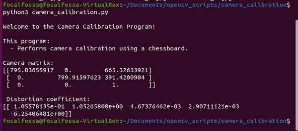
self.declare_parameter("camera_calibration_parameters_filename", "/home/focalfossa/dev_ws/src/opencv_tools/opencv_tools/calibration_chessboard.yaml")
self.declare_parameter("image_topic", "/video_frames")
self.declare_parameter("aruco_marker_name", "aruco_marker")
# Read parameters
aruco_dictionary_name = self.get_parameter("aruco_dictionary_name").get_parameter_value().string_value
self.aruco_marker_side_length = self.get_parameter("aruco_marker_side_length").get_parameter_value().double_value
self.camera_calibration_parameters_filename = self.get_parameter(
"camera_calibration_parameters_filename").get_parameter_value().string_value
image_topic = self.get_parameter("image_topic").get_parameter_value().string_value
self.aruco_marker_name = self.get_parameter("aruco_marker_name").get_parameter_value().string_value
# Check that we have a valid ArUco marker
if ARUCO_DICT.get(aruco_dictionary_name, None) is None:
self.get_logger().info("[INFO] ArUCo tag of '{}' is not supported".format(
args["type"]))
# Load the camera parameters from the saved file
cv_file = cv2.FileStorage(
self.camera_calibration_parameters_filename, cv2.FILE_STORAGE_READ)
self.mtx = cv_file.getNode('K').mat()
self.dst = cv_file.getNode('D').mat()
cv_file.release()
# Load the ArUco dictionary
self.get_logger().info("[INFO] detecting '{}' markers...".format(
aruco_dictionary_name))
self.this_aruco_dictionary = cv2.aruco.Dictionary_get(ARUCO_DICT[aruco_dictionary_name])
self.this_aruco_parameters = cv2.aruco.DetectorParameters_create()
# Create the subscriber. This subscriber will receive an Image
# from the video_frames topic. The queue size is 10 messages.
self.subscription = self.create_subscription(
Image,
image_topic,
self.listener_callback,
10)
self.subscription # prevent unused variable warning
# Initialize the transform broadcaster
self.tfbroadcaster = TransformBroadcaster(self)
# Used to convert between ROS and OpenCV images
self.bridge = CvBridge()
def listener_callback(self, data):
"""
Callback function.
"""
# Display the message on the console
self.get_logger().info('Receiving video frame')
# Convert ROS Image message to OpenCV image
current_frame = self.bridge.imgmsg_to_cv2(data)
# Detect ArUco markers in the video frame
(corners, marker_ids, rejected) = cv2.aruco.detectMarkers(
current_frame, self.this_aruco_dictionary, parameters=self.this_aruco_parameters,
cameraMatrix=self.mtx, distCoeff=self.dst)
# Check that at least one ArUco marker was detected
if marker_ids is not None:
# Draw a square around detected markers in the video frame
cv2.aruco.drawDetectedMarkers(current_frame, corners, marker_ids)
# Get the rotation and translation vectors
rvecs, tvecs, obj_points = cv2.aruco.estimatePoseSingleMarkers(
corners,
self.aruco_marker_side_length,
self.mtx,
self.dst)
# The pose of the marker is with respect to the camera lens frame.
# Imagine you are looking through the camera viewfinder,
# the camera lens frame's:
# x-axis points to the right
# y-axis points straight down towards your toes
# z-axis points straight ahead away from your eye, out of the camera
for i, marker_id in enumerate(marker_ids):
# Create the coordinate transform
t = TransformStamped()
t.header.stamp = self.get_clock().now().to_msg()
t.header.frame_id = 'camera_depth_frame'
t.child_frame_id = self.aruco_marker_name
# Store the translation (i.e. position) information
t.transform.translation.x = tvecs[i][0][0]
t.transform.translation.y = tvecs[i][0][1]
t.transform.translation.z = tvecs[i][0][2]
# Store the rotation information
rotation_matrix = np.eye(4)
rotation_matrix[0:3, 0:3] = cv2.Rodrigues(np.array(rvecs[i][0]))[0]
r = R.from_matrix(rotation_matrix[0:3, 0:3])
quat = r.as_quat()
# Quaternion format
t.transform.rotation.x = quat[0]
t.transform.rotation.y = quat[1]
t.transform.rotation.z = quat[2]
t.transform.rotation.w = quat[3]
# Send the transform
self.tfbroadcaster.sendTransform(t)
# Draw the axes on the marker
cv2.aruco.drawAxis(current_frame, self.mtx, self.dst, rvecs[i], tvecs[i], 0.05)
# Display image
cv2.imshow("camera", current_frame)
cv2.waitKey(1)
def main(args=None):
# Initialize the rclpy library
rclpy.init(args=args)
# Create the node
aruco_node = ArucoNode()
# Spin the node so the callback function is called.
rclpy.spin(aruco_node)
# Destroy the node explicitly
# (optional - otherwise it will be done automatically
# when the garbage collector destroys the node object)
aruco_node.destroy_node()
# Shutdown the ROS client library for Python
rclpy.shutdown()
if __name__ == '__main__':
main()
Save the file, and close it.
Open the package.xml file by opening a new terminal window, and typing:
cd ~/dev_ws/src/opencv_tools/
gedit package.xml
Add the following lines to the package.xml file in the appropriate location.
<depend>geometry_msgs</depend>
<depend>tf2_ros</depend>
<depend>tf_transformations</depend>
Save the file, and close it.
Now open the setup.py file.
gedit setup.py
Add the following line under the ‘img_subscriber’ = …. line.
'aruco_marker_pose_estimator_tf = opencv_tools.aruco_marker_pose_estimation_tf:main',
Save the file, and close it.
Build the package:
cd ~/dev_ws/
colcon build
Run the Nodes
To run the nodes, open a new terminal window.
Make sure you are in the root of your workspace:
cd ~/dev_ws/
Run the image publisher node. If you recall, its name is img_publisher.
ros2 run opencv_tools img_publisher
Open a new terminal window, and type:
ros2 run opencv_tools img_publisher
Open another terminal window, and type:
ros2 run opencv_tools aruco_marker_pose_estimator_tf
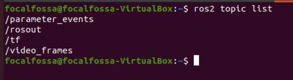
Let’s check out the topics.
ros2 topic list
Let’s see the tf topic.
ros2 topic echo /tf
How to Visualize an ArUco Marker Pose in RViz
Now open a new terminal window, and type:
rviz2
Change the Fixed Frame to camera_depth_frame.
Click the Add button on the bottom-left.
Scroll down to TF and add the TF plugin.
You should see the following output.


