What are Deep Learning Methods Really Learning?

It is not exactly clear what deep learning methods are really learning. Sure, they are highly effective and are learning something, but I’m still trying to get my head around exactly what they are learning.

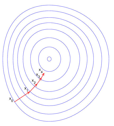
Consider your run-of-the-mill deep neural network. “Learning” is nothing more than an optimization procedure. We are trying to produce an optimized mathematical formula that takes in a set of training examples and then can, as accurately as possible, map the inputs (i.e. attributes, features, etc.) of those examples to the outputs (i.e. class, target variable, etc.). We then use this formula to classify a new set of examples.
gradient_descent_png
Gradient Descent. Is this really all there is to learning?

At its core, deep learning is about input-process-output. It is not true learning in the sense of the word (the way we humans do). True learning entails understanding, and understanding is nonexistent during deep learning. 

You can memorize a book, chapter-by-chapter, word-for-word; but that doesn’t mean you are learning. You still would not understand the plot. Similarly, in deep learning there is no understanding. Deep learning “memorizes” a mapping between inputs and outputs without any real understanding of the why behind those relationships. And in my view, the why is a huge part of learning. True learning (in the human sense of the word) without understanding is not learning. Perhaps then we should call deep learning something different? Deep optimization perhaps??? Guess that didn’t sound as marketable and sexy as deep learning.

If you look out in nature — the human brain or the brain of any living organism — nothing out there learns in a way that even remotely resembles backpropagation. Neural networks are about classification error, but real learning — the way humans learn — is deeper than that (pun intended). 

A neural network, for example, has a completely different concept of what it is to be a dog. That concept could involve where certain groups of pixels are placed and may have nothing to do with the actual structure of the animal. Where a human would see legs, arms, torso, etc., a deep learning algorithm may abstract a completely different set of things. This has led a rise in adversarial attacks, where an attacker is able to determine what representation provides the highest probability for an image to be classified as anything and is able to insert noise that causes things to be misclassified.

Another point to consider is that neural networks generate something. It may be a relationship that we did not previously understand, but it may also just be nonsense that happens to work.  The abstractions may result in some representational form that is at its most basic just complete nonsense. If there is no real understanding of what the abstractions that the algorithm makes, then it is hard to confirm that it’s actually doing anything.
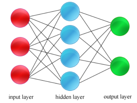
neural_network
A Basic Neural Network

The significance of the lack of understanding of what deep learning is, is yet to be seen; but here are just a few of the consequences if the hype gets unchecked:

  • Wasted resources as venture capitalists throw money at anything that has to do with deep learning. 
  • Wasted resources as non-expert government agencies fund any research project that has the term “deep learning” in it.
  • A boat load of computer science graduates around the world that, all of a sudden, have found their “passion” in deep learning.
  • Disappointed companies as deep learning does not have the expected impact on their bottom line.
  • Another AI winter.

Remember, there is the marketing element in there too. Using anthropomorphic terms like machine “learning” and deep “learning” is a much better sell to a general audience than machine mathematical optimization or deep optimization. Researchers gotta sell their ideas too!

Bottom Line: Artificial intelligence is not yet intelligent, and deep learning is not yet deep (yay! we still have work to do!)…nor is it learning in the true sense of the word. Deep learning certainly will continue to have an enormous impact on the world, but there needs to be more awareness and discussion of not just the enormous potential of deep learning but also its limitations so non-technical stakeholders can make more informed decisions.

Why Deep Learning Has Received So Much Attention Lately

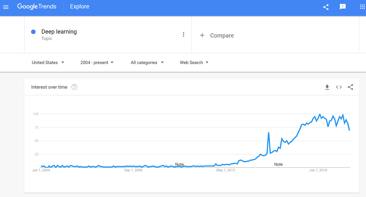
Deep learning has been receiving an enormous amount of interest over the last seven years in the academic and business communities. Let’s take a look at the definition of deep learning, and then we will take a look at how this field has become so popular so quickly.

What is Deep Learning

Deep learning is a machine learning technique in which we teach a computer how to make predictions. Predictions are made by mapping a set of inputs to a set of outputs. 

Input Data —–> Deep Learning Algorithm (i.e. Process) —–> Output Data

For example, let’s say our input data into a deep learning algorithm is a set of photos. We want to be able to automatically tag each photo as either being dogs or elephants.

dogs_playing_on_beach
Dogs
elephant_flock_baby_elephant
Elephants

Input Data (lots of images containing dogs and elephants) —–> Deep Learning Algorithm —–> Classification of Each Image (i.e. Dogs or Elephants)

The “learning” part of the term deep learning entails looking at a bunch (hundreds, thousands, even millions+) of photos of elephants and dogs to develop a mathematical model of what both animals look like. Once the deep learning algorithm has been trained to recognize dogs and elephants, it can then be used to classify new photos as either dogs or elephants.

Most deep learning algorithms use neural network architectures as the structure of the underlying mathematical model. For this reason, deep learning methods are commonly called deep neural networks. 

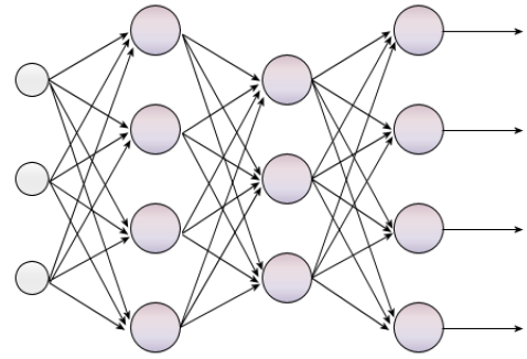
Neural networks consist of layers and interconnected nodes. The first layer is the input layer. This layer might consist of, for example, thousands of matrices of pixels that represent photos of dogs or elephants. Each layer after the input layer transforms the data slightly so that the data is more abstract and complete than the previous layer. 

The layer after the input layer (i.e. second layer), for example, might contain nodes that recognize simple shapes like circles and edges (that at this point look nothing like a dog or elephant). The third layer contains nodes that recognize more complex shapes that look like a dog’s body parts (e.g. nose, eye, ear, etc.). Then the final layer, the output layer, outputs the classification of a photo as being either a dog or elephant.

neural-network
A basic multi-layer neural network architecture. The first layer on the left is the input layer. The two inner layers of nodes (neurons) are the hidden layers. The fourth layer on the right is the output layer that outputs the classification. In this case, the network expects four different classes in the data set (e.g. dogs, elephants, cows, horses).

Forbes Magazine has a good image showing the basic deep neural network structure I described above.

The “deep” part of deep learning refers to the number of hidden layers in the neural network. Standard neural networks have two or three (like in my example above) hidden layers, but deep neural networks can have 100+ layers. 

In short, a deep neural network is one that has several hidden layers, with the idea that these layers learn different levels of abstraction of the input attributes; thereby allowing the network to solve more complex problems, such as face recognition, object tracking and so on.

Origin of the Deep Learning Revolution: AlexNet

This post at Medium.com shows the graphs of the percentage of selected arXiv publications with either “deep”, “adversarial” or “convolutional” in the title. Note how the graph was virtually all 0s prior to 2010. It then took off like a rocket in 2012. What happened in 2012?

In 2010 and 2011, Fei-Fei Li held the ImageNet competition, an annual machine learning contest. Contest participants were given millions of images to use to train their models. These images were pre-labeled with one of ~1,000 different categories (e.g. leopard, cherry, mushroom, etc.). The objective of the contest was to correctly classify examples that were not in the training set. 

During those first two years of the competition in 2010 and 2011, the winning teams had a classification accuracy of 72%. None of the winners of those competitions used deep learning methods. Then in 2012, a team from the University of Toronto led by Alex Krizhevsky won the competition with a classification accuracy of 84%. The second place contestant had a classification accuracy of 74%. The team from the University of Toronto used deep learning methods combined with the computational power of graphical processing units (GPUs) to completely blow the competition out of the water.

The results were remarkable and gave birth to the deep learning era that continues to this day.

Why Deep Learning Has Received So Much Attention Lately

With traditional machine learning approaches, you would have to design a feature extraction algorithm which generally involves a lot of heavy mathematics (complex design), may not be very efficient, and does not perform well (i.e. accuracy may not be suitable for real-world applications). After doing all of that, you would also have to design a whole classification model to classify your input given the extracted features (i.e. attributes).

That’s a lot of work!

Enter Deep Learning…

  • With deep neural networks, we can perform feature extraction and classification in one shot, which means we could only need to design one model.
  • The availability of large amounts of labeled data as well as GPUs, which can process data in parallel at high speeds, enables these models to be much faster than previous methods.
  • Using the back-propagation algorithm, a well-designed loss function, and millions of parameters, these deep networks are able to learn highly complex features (which had to traditionally be hand designed)…i.e. no more complex design!
  • Deep neural networks have become fairly easy to implement with high-level open source libraries such as Keras, Pytorch, and TensorFlow.

Deep Learning has made many new applications practically feasible. We wouldn’t have been able to make good language translators pre-deep learning, because we simply had no technique at the time that would perform well enough or at a high enough speed for a real-world application.  Deep learning techniques have been applied to not just image recognition, but automatic speech recognition, natural language processing, drug discovery, customer relationship management, robotics, self-driving cars, and more.

How to Choose an Optimal Learning Rate for Gradient Descent

One of the challenges of gradient descent is choosing the optimal value for the learning rate, eta (η). The learning rate is perhaps the most important hyperparameter (i.e. the parameters that need to be chosen by the programmer before executing a machine learning program) that needs to be tuned (Goodfellow 2016).

If you choose a learning rate that is too small, the gradient descent algorithm might take a really long time to find the minimum value of the error function. This defeats the purpose of gradient descent, which was to use a computationally efficient method for finding the optimal solution.

On the other hand, if you choose a learning rate that is too large, you might overshoot the minimum value of the error function, and may even never reach the optimal solution. 

Before we get into how to choose an optimal learning rate, it should be emphasized that there is no value of the learning rate that will guarantee convergence to the minimum value of the error function (assuming global) value of a function. 

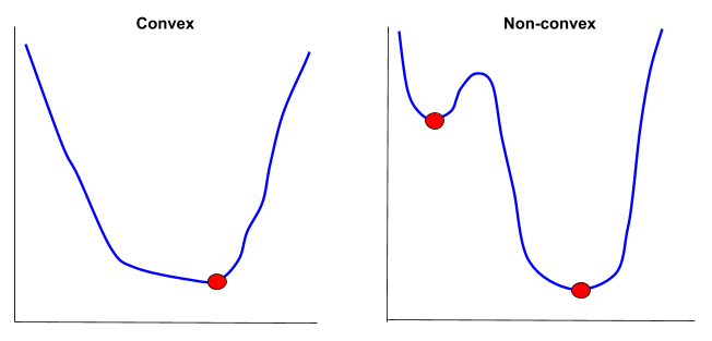
Algorithms like logistic regression are based on gradient descent and are therefore what is known as “hill climber.” Therefore, for non-convex problems (where the graph of the error function contains local minima and a global minimum vs. convex problems where global minimum = local minimum), they will most likely get stuck in a local minimum. 

convex-vs-nonconvex-graphs

So with that background, we are ready to take a look at some options for selecting the optimal learning rate (eta) for gradient descent.

Choose a Fixed Learning Rate

The standard gradient descent procedure uses a fixed learning rate (e.g. 0.01) that is determined by trial and error. For example:

“Typical values for a neural network with standardized inputs (or inputs mapped to the (0,1) interval) are less than 1 and greater than 10-6 but these should not be taken as strict ranges and greatly depend on the parametrization of the model. A default value of 0.01 typically works for standard multi-layer neural networks but it would be foolish to rely exclusively on this default value. If there is only time to optimize one hyper-parameter and one uses stochastic gradient descent, then this is the hyper-parameter that is worth tuning.”

Bengio (2013)

Use Learning Rate Annealing

Learning rate annealing entails starting with a high learning rate and then gradually reducing the learning rate linearly during training. The learning rate can decrease to a value close to 0.

The idea behind this method is to quickly descend to a range of acceptable weights, and then do a deeper dive within this acceptable range.

Use Cyclical Learning Rates

Cyclical learning rates have been proposed: 

“Instead of monotonically decreasing the learning rate, this method lets the learning rate cyclically vary between reasonable boundary values.”

Leslie (2017)

Use an Adaptive Learning Rate

Another option is to use a learning rate that adapts based on the error output of the model. Here is what the experts say about adaptive learning rates.

Reed (1999) notes on page 72 of his book Neural Smithing: Supervised Learning in Feedforward Artificial Neural Networks that an adaptable learning rate is preferred over a fixed learning rate:

“The point is that, in general, it is not possible to calculate the best learning rate a priori. The same learning rate may not even be appropriate in all parts of the network. The general fact that the error is more sensitive to changes in some weights than in others makes it useful to assign different learning rates to each weight”

Reed (1999)

Melin et al. (2010) writes:

“First, the initial network output and error are calculated. At each epoch new weights and biases are calculated using the current learning rate. New outputs and errors are then calculated.

As with momentum, if the new error exceeds the old error by more than a predefined ratio (typically 1.04), the new weights and biases are discarded. In addition, the learning rate is decreased. Otherwise, the new weights, etc. are kept. If the new error is less than the old error, the learning rate is increased (typically by multiplying by 1.05).”

Melin et al. (2010)

References

Bengio, Y. Practical Recommendations for Gradient-based Training of Deep Architectures. In K.-R. Muller, G. Montavon, and G. B. Orr, editors, Neural Networks: Tricks of the Trade. Springer, 2013.

Goodfellow, Ian, Yoshua Bengio, and Aaron Courville. Deep Learning. Cambridge, Massachusetts: The MIT Press, 2016. Print.

Melin, Patricia, Janusz Kacprzyk, and Witold Pedrycz. Soft Computing for Recognition Based on Biometrics. Berlin Heidelberg: Springer, 2010. Print.

Reed, Russell D., and Robert J. Marks. Neural Smithing: Supervised Learning in Feedforward Artificial Neural Networks. Cambridge, Mass: MIT Press, 1999. Print.

Smith, Leslie N. Cyclical learning rates for training neural networks. In Applications of Computer Vision (WACV), 2017 IEEE Winter Conference on. IEEE, pages 464–472.