

One of the challenges of gradient descent is choosing the optimal value for the learning rate, eta (η). The learning rate is perhaps the most important hyperparameter (i.e. the parameters that need to be chosen by the programmer before executing a machine learning program) that needs to be tuned (Goodfellow 2016).
If you choose a learning rate that is too small, the gradient descent algorithm might take a really long time to find the minimum value of the error function. This defeats the purpose of gradient descent, which was to use a computationally efficient method for finding the optimal solution.
On the other hand, if you choose a learning rate that is too large, you might overshoot the minimum value of the error function, and may even never reach the optimal solution.
Before we get into how to choose an optimal learning rate, it should be emphasized that there is no value of the learning rate that will guarantee convergence to the minimum value of the error function (assuming global) value of a function.
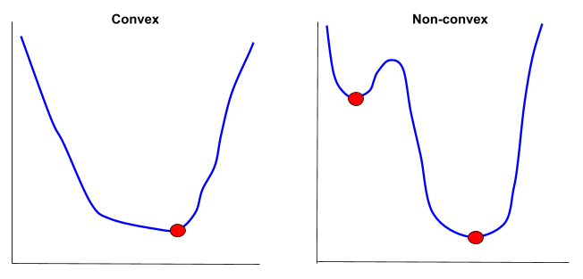
Algorithms like logistic regression are based on gradient descent and are therefore what is known as “hill climber.” Therefore, for non-convex problems (where the graph of the error function contains local minima and a global minimum vs. convex problems where global minimum = local minimum), they will most likely get stuck in a local minimum.
So with that background, we are ready to take a look at some options for selecting the optimal learning rate (eta) for gradient descent.
Choose a Fixed Learning Rate
The standard gradient descent procedure uses a fixed learning rate (e.g. 0.01) that is determined by trial and error. For example:
“Typical values for a neural network with standardized inputs (or inputs mapped to the (0,1) interval) are less than 1 and greater than 10-6 but these should not be taken as strict ranges and greatly depend on the parametrization of the model. A default value of 0.01 typically works for standard multi-layer neural networks but it would be foolish to rely exclusively on this default value. If there is only time to optimize one hyper-parameter and one uses stochastic gradient descent, then this is the hyper-parameter that is worth tuning.”
Bengio (2013)
Use Learning Rate Annealing
Learning rate annealing entails starting with a high learning rate and then gradually reducing the learning rate linearly during training. The learning rate can decrease to a value close to 0.
The idea behind this method is to quickly descend to a range of acceptable weights, and then do a deeper dive within this acceptable range.
Use Cyclical Learning Rates
Cyclical learning rates have been proposed:
“Instead of monotonically decreasing the learning rate, this method lets the learning rate cyclically vary between reasonable boundary values.”
Leslie (2017)
Use an Adaptive Learning Rate
Another option is to use a learning rate that adapts based on the error output of the model. Here is what the experts say about adaptive learning rates.
Reed (1999) notes on page 72 of his book Neural Smithing: Supervised Learning in Feedforward Artificial Neural Networks that an adaptable learning rate is preferred over a fixed learning rate:
“The point is that, in general, it is not possible to calculate the best learning rate a priori. The same learning rate may not even be appropriate in all parts of the network. The general fact that the error is more sensitive to changes in some weights than in others makes it useful to assign different learning rates to each weight”
Reed (1999)
Melin et al. (2010) writes:
“First, the initial network output and error are calculated. At each epoch new weights and biases are calculated using the current learning rate. New outputs and errors are then calculated.
As with momentum, if the new error exceeds the old error by more than a predefined ratio (typically 1.04), the new weights and biases are discarded. In addition, the learning rate is decreased. Otherwise, the new weights, etc. are kept. If the new error is less than the old error, the learning rate is increased (typically by multiplying by 1.05).”
Melin et al. (2010)
References
Bengio, Y. Practical Recommendations for Gradient-based Training of Deep Architectures. In K.-R. Muller, G. Montavon, and G. B. Orr, editors, Neural Networks: Tricks of the Trade. Springer, 2013.
Goodfellow, Ian, Yoshua Bengio, and Aaron Courville. Deep Learning. Cambridge, Massachusetts: The MIT Press, 2016. Print.
Melin, Patricia, Janusz Kacprzyk, and Witold Pedrycz. Soft Computing for Recognition Based on Biometrics. Berlin Heidelberg: Springer, 2010. Print.
Reed, Russell D., and Robert J. Marks. Neural Smithing: Supervised Learning in Feedforward Artificial Neural Networks. Cambridge, Mass: MIT Press, 1999. Print.
Smith, Leslie N. Cyclical learning rates for training neural networks. In Applications of Computer Vision (WACV), 2017 IEEE Winter Conference on. IEEE, pages 464–472.