In this post, I will explore the idea of latent variable models, where a latent variable is a “hidden” variable (i.e., one we cannot observe directly but that plays a part in the overall model).

Table of Contents

What is a Latent Variable?

A latent variable is a variable that is not directly observed but is inferred from other variables we can measure directly.

A common example of a latent variable is quality of life. You cannot measure quality of life directly.

Real-world Example of Latent Variables

A few years ago, my wife and I decided to move cities to a place which would be able to offer us a better quality of life. I created a spreadsheet in Excel containing all the factors that influence the quality of life in a particular location. They are:

Days per year of sunshine
Unemployment rate
Crime rate
Average household income
State income tax rate
Cost of living
Population density
Median home price
Average annual temperature
Number of professional sports teams
Average number of days of snow per year
Population
Average inches of rain per year
Number of universities
Distance to an international airport

If I wanted to feed this into a machine learning algorithm, I could then develop a mathematical model for quality of life.

The advantage of using the latent variable model with quality of life is that I can use a fewer number of features, which reduces the dimensionality of what would be an enormous data set. All those factors I mentioned are correlated in some way to the latent variable quality of life. So instead of using 15 columns of data, I can use just 1. The data then becomes not only easier to understand but useful if I want to use a quality of life score as a feature for any type of classification or regression problem because it captures the underlying phenomenon we are interested in.

Exploring the Use of Latent Variables Across Different Model Types

One particularly useful framework for exploring the use of latent variables across different model types is the idea of path analysis. In path analysis, one develops a model that shows the relationships between variables that we can readily measure and variables that we cannot readily measure. These variables that we cannot readily measure are called latent variables.

By convention, variables that we can readily measure will be placed inside rectangles or boxes. Variables that we cannot readily measure, the latent variables, are typically located inside ovals.

Let’s look at an example now of how we can model latent variables using the latent variable of childhood intelligence.

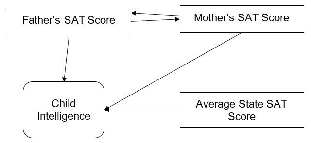
As you can see in this diagram we have four different boxes.

We have the oval at the bottom which is representative of the intelligence of a child. This is the latent variable. This is the variable that we want to predict.

Then up above we have two boxes. One box includes the father’s SAT score. The other box is the mother’s SAT score. And then finally we have another box which represents the average SAT scores of students in the state that the child lives in.

Note that in this particular path model, we draw arrows showing relationships between two variables. The arrow between the father and the mother is indicative of correlation. We are inferring in this particular model a correlation between the SAT score of the father and the SAT score of the mother, and we are also inferring a relationship between both of their SAT scores and the intelligence of a child.

We are also showing a correlation relationship between the average SAT score of the students in the state and the child’s intelligence.

But notice that there are no arrows that are drawn from either the father or the mother to the average SAT scores in the state. The lack of arrows is indicative of a lack of correlation between those two variables.

In short, I believe at the outset of a machine learning problem, we can draw different path models to begin to model the relationships and to develop an appropriate framework for selecting a model to tackle a particular machine learning problem.

Getting back to the idea of path modeling that I described earlier, we can use this diagram to not only explore the relationship between observed variables and latent variables, but we could use it as a springboard to actually develop quantifiable relationships between observed and latent variables…in other words, the numerical coefficients that we can use as inputs into a particular mathematical model.

Let’s take a look at an example, perhaps the simplest example we can think of…the equation for a line of best fit:

y = mx + b.

You might recall the equation y = mx + b from grade school. In this particular equation, y is the dependent variable, b is the intercept, m is the slope, and x is the independent variable.

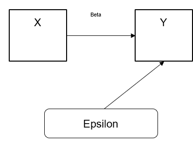
In a linear regression model we typically see an equation of the form:

Y = (BETA) * X + EPSILON

where EPSILON is the “residual”, the difference between actual and predicted values for a given value for x.

What would a path diagram look like for this example?

Let’s draw it.

I think this is a very cool way of being able to very easily take a very large data set and begin to think of ways of how we can condense this data set into a data set which would have lower storage requirements. By adding weightings to the arrows and by following the actual arrows that show the correlations between two variables whether observed or unobserved, we can then use this as an outline to start pruning irrelevant features from the data set. The next step would be able to use the subset of features to develop a hopefully useful predictive model with one of the common machine learning models available.

Factor Analysis

One framework for generating latent variable models is the idea of factor analysis.

In factor analysis, we want to determine if the variations in the measured, observed variables are primarily the result of variations in the underlying latent variables. We can then use this information, the interdependencies between the latent variables and the observed variables, to eliminate some of the features in our data set and therefore reduce the storage requirements for a particular machine learning problem. We do this by estimating the covariance (the extent to which two variables move in tandem with each other) between the observed variables and the unobserved latent variables.

Why is this promising? It is promising because we can create models of things we want to measure but are not easily able to measure. And in doing that, we can tackle the representation bias inherent in many decisions made by human beings.

Real-World Example of Factor Analysis

Let’s look at a concrete example to see how all of this fits together and how it would be implemented in the real world.

Imagine we are a software engineering team at a big company trying to hire employees that have “outstanding” technical ability. “Technical ability,” like the terms altruism, generosity, health, creativity, aggressiveness, and innovativeness, are all terms that are not easily quantifiable or measured. So let us consider the term technical ability a latent variable.

We can then consider some observed variables as part of the candidate evaluation process:

Number of lines of code written
Kaggle scores
Hacker rank
Grade point average
SAT score
GRE score
Number of years of experience

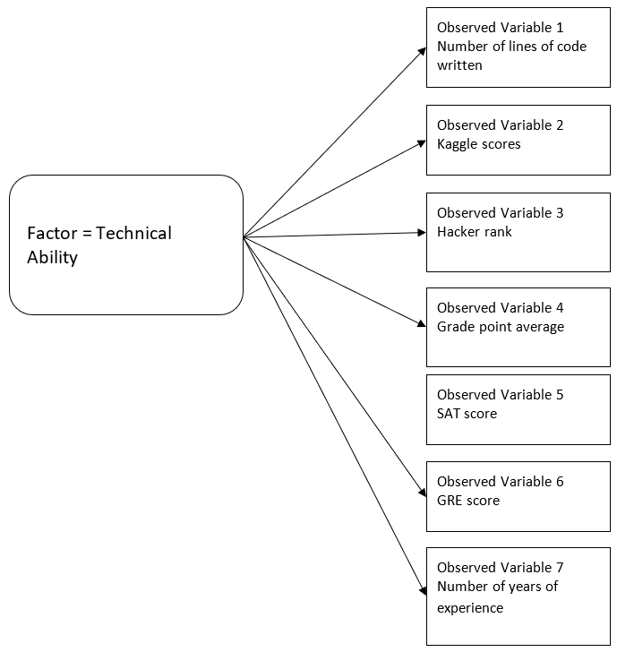
These would be all of the observed variables that we believe are connected in some way to the underlying factor known as technical ability.

At the end of the day, technical ability is what we would like to discover, but since we can’t measure that directly , we use data from some other variables in order to back in to that technical ability. And if you see on each of these arrows, we could add additional weightings to our model to be able to determine which of the particular observed variables we can safely remove from the model and still achieve a result that is desirable that gets us a candidate that has the technical ability we want.

So you can see by having some kind of model developed by factor analysis, we can help eliminate some of the representation bias that might be evident in a hiring system.

At the end of the day, people who hire teams of software engineers have their own inherent bias about who to hire and who not to hire. These biases might be based on irrelevant factors such as the hiring manager’s experience with people who looked similar to the candidate, how the candidate speaks, etc.

By evaluating the results of a model that is based on mathematics, we can then compare the results of the model to individual opinions in the team to try to get a more appropriate result and hire the best candidate…all the while alleviating any concerns of representative bias that might exist in the hiring process.