The inverse kinematics problem in robotics asks the following question: What do the angles of the servo motors need to be given our desired position and orientation of the end effector of a robotic arm (e.g. gripper, hand, vacuum suction cup, etc.)?
You can see how this problem has all sorts of real-world applications. For example, imagine we have a robotic arm that is inside a warehouse. We want the robotic arm to pick up items that are in one location and place them in another (i.e. pick and place).

This problem is exactly the inverse kinematics problem. We know where we want the robotic arm to go, and we need to solve for the joint variables (e.g. servo motor angles) so that we can command the robotic arm’s end effector to the correct location to pick up the items.
In this tutorial, I will cover one way to solve the inverse kinematics problem. It is called the graphical approach. The graphical approach depends on us using trigonometry to solve for the values of the joint variables given the desired position of the end effector.
The graphical approach to inverse kinematics is useful for robotic arms with three degrees of freedom or less. Beyond three degrees of freedom, we need to use another approach, which I will cover in a future tutorial.
Example 1 – Two Degree of Freedom Robotic Arm: Revolute + Prismatic
Consider the following kinematic diagram of a two degree of freedom robotic arm. We have a revolute joint (i.e. regular servo motor with rotation motion) at the base of the arm. This revolute joint is connected to a prismatic joint (i.e. a linear actuator that produces linear motion).
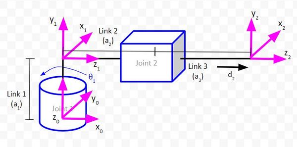
For this robotic arm above, we want to be able to tell it where the end effector (frame 2 above…x2, y2, z2 coordinate axes) should go. To accomplish this, we need to have trigonometric equations in place that enable us to solve for the joint variables (e.g. servo angle for Joint 1 and linear actuator displacement for Joint 2) given our desired end effector position.
Draw the Kinematic Diagram From Either an Aerial View or Side View
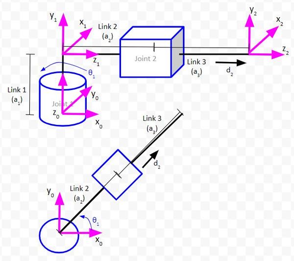
Let’s start by drawing the kinematic diagram from an aerial view. That is, we want to look down on the plane created by the x0 and y0 axes.
We will let θ1 = 45 degrees. This angle will make it easier for us to draw the triangles (i.e. trigonometry) we need to solve the inverse kinematics.
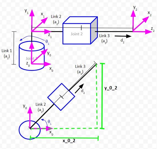
Let’s start by drawing the kinematic diagram from an aerial view. That is, we want to look down on the plane created by the x0 and y0 axes.
We will let θ1 = 45 degrees. This angle will make it easier for us to draw the triangles (i.e. trigonometry) we need to solve the inverse kinematics.
Sketch Triangles on Top of the Kinematic Diagram
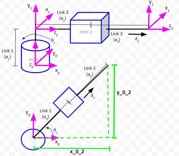
The first triangle we will draw enables us to determine the position of the end effector (i.e. the origin of coordinate frame 2) relative to the position of the base frame (i.e. the origin of coordinate frame 0).
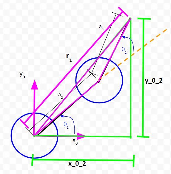
The side of the triangle that is parallel to the vector y0 will be labeled as y_0_2. This distance represents the y position of the end effector relative to the base frame of the robotic arm.
The side of the triangle that is parallel to the vector x0 will be labeled as x_0_2. This distance represents the x position of the end effector relative to the base frame of the robotic arm.
The Three Useful Trigonometric Relationships
There are three trigonometric relationships that will help us solve the inverse kinematics for this robotic arm. Solving the inverse kinematics means finding the values for each joint variable.
1. Pythagorean Theorem: a2 + b2 = c2
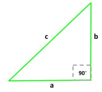
2. SOHCAHTOA
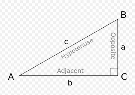
This trigonometric relationship says that given a right triangle with angle A and sides a, b, and c:
- sin A = opposite/hypotenuse = a/c
- cos A = adjacent/hypotenuse = b/c
- tan A = opposite/adjacent = a/b
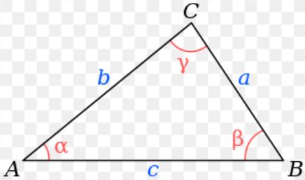
The law of cosines is a generalized form of the Pythagorean theorem. It works for right triangles as well as for non-right triangles. The three relationships are as follows
- a2 = b2 + c2 – 2bccosα
- b2 = a2 + c2 – 2accosβ
- c2 = a2 + b2 – 2abcosγ
Solve for d2
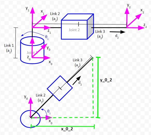
To solve for d2, we need to select one of the three trigonometric relationships. Let’s use the Pythagorean theorem. We have:
(x_0_2)2 + (y_0_2)2 = (a2 + a3 + d2)2
In the equation above, the only unknown value is d2 because we know the link lengths (a2 and a3), and x_0_2 and y_0_2 represent the position of the end effector that we desire. The displacement of the linear actuator (d2) is what we want to know.
Let’s solve for d2.
square_root((x_0_2)2 + (y_0_2)2) = (a2 + a3 + d2)
(a2 + a3 + d2) = square_root((x_0_2)2 + (y_0_2)2)
d2 = square_root((x_0_2)2 + (y_0_2)2) – a2 – a3
Making the above equation look prettier, we have:

Solve for θ1
Now, let’s solve for the other unknown, the value of θ1. Looking at my three useful trigonometric relationships, SOHCAHTOA looks like it will help us.
tan θ1 = opposite/adjacent = y_0_2 / x_0_2
Therefore,
θ1 = tan-1(y_0_2 / x_0_2)
Making it look prettier, we have:

We are done because we have equations for both joint variables.
Example 2 – Two Degree of Freedom Robotic Arm: Revolute + Revolute
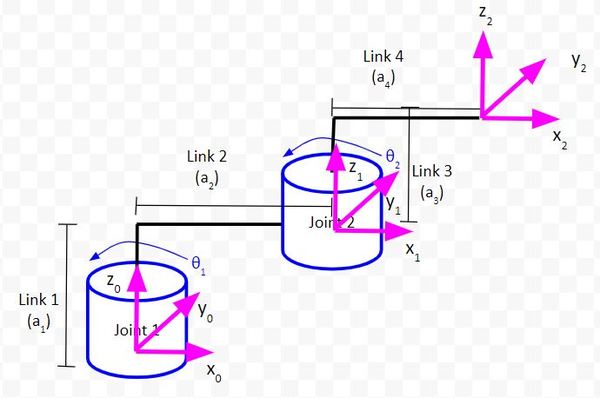
Let’s look at another example. We’ll work out the inverse kinematics for the two degree of freedom robotic arm that we built in a previous tutorial.
Draw the Kinematic Diagram From Either an Aerial View or Side View
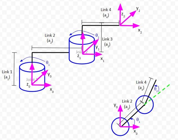
Sketch Triangles on Top of the Kinematic Diagram
Let’s draw the first triangle in green.
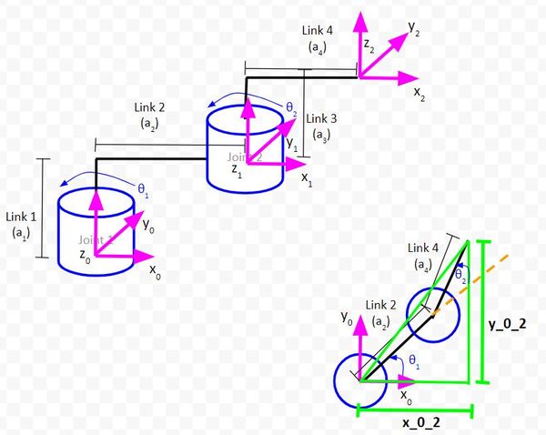
Let’s zoom in and draw another triangle. We’ll make this one pink.
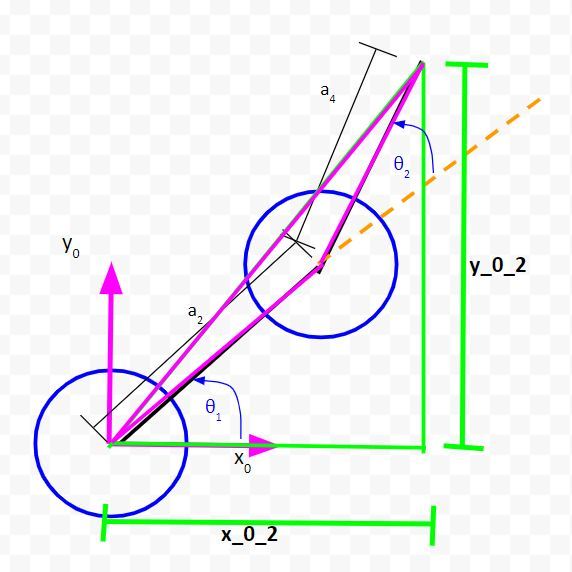
Let the long side of the triangle we just created be r1.
Solve for the Unknown Variables
Solve for r1
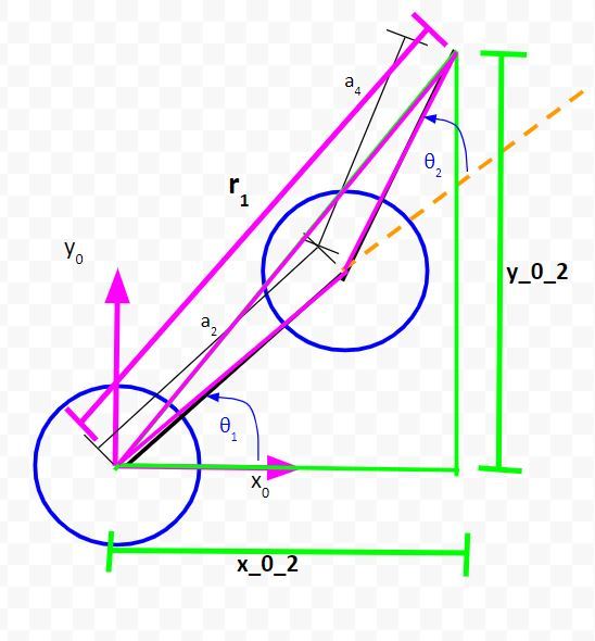
Let’s start by looking at the green right triangle above. To solve for r1, we can use the Pythagorean Theorem.
r12 = (x_0_2)2 + (y_0_2)2
Take the square root of both sides. We’ll label this as equation 1…
(1) r1 = square_root((x_0_2)2 + (y_0_2)2)
Solve for θ1
Now let’s look at the pink triangle. Because this isn’t a right triangle, we’ll have to use the law of cosines.
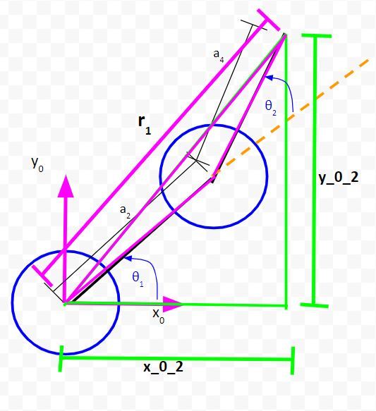
To use the law of cosines and to solve for θ1, we need to label some angles.
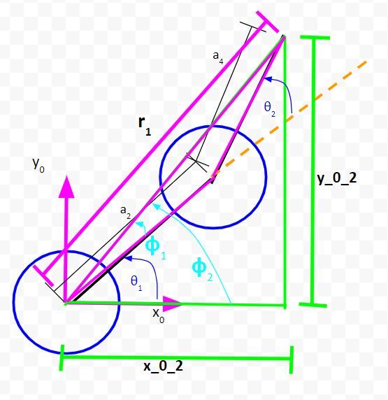
I have added two new angles, ϕ1 and ϕ2.
We can see from the diagram that:
θ1 = ϕ2 – ϕ1
Using the law of cosines, we have:
a42 = r12 + a22 – 2r1a2cos(ϕ1)
Now, solve for ϕ1. This will be equation #2.
(2) ϕ1 = arccos((a42 – r12 – a22)/(-2r1a2))
Also, we can see from the diagram that…
(3) ϕ2 = arctan((y_0_2) / (x_0_2))
Now that we have expressions for ϕ1 and ϕ2, we can solve for θ1.
(4) θ1 = ϕ2 – ϕ1
Solve for θ2
To solve for θ2, we need to label yet another angle. I’ll label that obtuse angle in the pink triangle ϕ3.
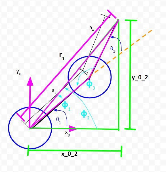
Look at the diagram above. You can see that:
ϕ3 + θ2 = 180°
Therefore,
θ2 = 180° – ϕ3
To find the value of ϕ3, we need to use the law of cosines.
r12 = a22 + a42 – 2a2a4cos(ϕ3)
Solving for ϕ3, we get…
(5) ϕ3 = arccos((r12 – a22 – a42)/(-2a2a4))
Now, we can solve for θ2…
(6) θ2 = 180° – ϕ3
Put It All Together
Now, let’s gather all our useful equations together:
(1) r1 = square_root((x_0_2)2 + (y_0_2)2)
(2) ϕ1 = arccos((a42 – r12 – a22)/(-2r1a2))
(3) ϕ2 = arctan((y_0_2) / (x_0_2))
(4) θ1 = ϕ2 – ϕ1
(5) ϕ3 = arccos((r12 – a22 – a42)/(-2a2a4))
(6) θ2 = 180° – ϕ3
Implement Inverse Kinematics for a Real Robotic Arm
Now that we’ve derived all our equations, let’s see all this math in action on a real robot. We want to be able to specify an (x,y) coordinate where we want the end effector of the robot to go to. The robotic arm will then move to that location.
To complete this section, you need to have completed this tutorial.
When we created code for the forward kinematics of this robotic arm, we set both joint angles to 45 degrees. We then ran the code, and the end effector of the robotic arm moved to the (x = 4 cm, y = 10 cm) position on the dry erase board.
Since we are doing the inverse kinematics problem, we will now do everything in reverse. We will tell the robot to move the end effector to the (x = 4 cm, y = 10 cm) position on the dry erase board. The code we will write will automatically calculate the joint angles that will make that motion happen.
Let’s open a new sketch in the Arduino IDE. We’ll call this program ik_2dof_robotic_arm_v1.ino.
Here is the code:
/*
Program: Inverse Kinematics on a Two Degree of Freedom Robotic Arm (Graphical Method)
File: ik_2dof_robotic_arm_v1.ino
Description: This program is an implementation of inverse kinematics for
  a two degree of freedom robotic arm. Given a desired x and y position
  for the end effector, the servo angles are calculated and then set.
Author: Addison Sears-Collins
Website: https://automaticaddison.com
Date: August 26, 2020
*/

#include <VarSpeedServo.h>

// Define the number of servos
#define SERVOS 2

// Create the servo objects.
VarSpeedServo myservo[SERVOS];

// Speed of the servo motors
// Speed=1: Slowest
// Speed=255: Fastest.
const int desired_speed = 75;

// Attach servos to digital pins on the Arduino
int servo_pins[SERVOS] = {3,5};

// Desired x and y position of the end effector
double x_pos = 4.0;
double y_pos = 10.0;

// Link lengths in centimeters
const double a1 = 4.7;
const double a2 = 5.9;
const double a3 = 5.4;
const double a4 = 6.0;

// Define the inverse kinematics variables
double r1 = 0.0;
double phi_1 = 0.0;
double phi_2 = 0.0;
double phi_3 = 0.0;
double theta_1 = 0.0;
double theta_2 = 0.0;

void setup() {

  // Set the baud rate for the serial port at 9600 bps
  // Used for trouble shooting
  //Serial.begin(9600);

  // Attach the servos to the servo object
  // attach(pin, min, max  ) - Attaches to a pin
  //   setting min and max values in microseconds
  //   default min is 544, max is 2400
  // Alter these numbers until both servos have a
  //   180 degree range.
  myservo[0].attach(servo_pins[0], 544, 2475);
  myservo[1].attach(servo_pins[1], 500, 2475);

  // Set initial servo positions
  myservo[0].write(0, desired_speed, true);
  myservo[1].write(calc_servo_1_angle(0), desired_speed, true);

  // Wait one second to let servos get into position
  delay(1000);
}

void loop() {

    /* Calculate the inverse kinematics*/
    // (1) r1  = square_root((x_0_2)^2 + (y_0_2)^2)
    // Value is in centimeters
    r1 = sqrt((x_pos * x_pos) + (y_pos * y_pos));

    // (2) ϕ1 = arccos((a4^2 - r1^2 - a2^2)/(-2*r1*a2))
    // The returned value is in the range [0, pi] radians.
    phi_1 = acos(((a4 * a4) - (r1 * r1) - (a2 * a2))/(-2.0 * r1 * a2));

    // (3) ϕ2 = arctan((y_0_2) / (x_0_2))
    // The atan2() function computes the principal value of the
    // arc tangent of y/x, using the signs of both arguments to
    // determine the quadrant of the return value.
    // The returned value is in the range [-pi, +pi] radians.
    phi_2 = atan2(y_pos,x_pos);

    // (4) θ1 =  ϕ1 - ϕ2
    // Value is in radians
    theta_1 = phi_2 - phi_1;

    // (5) ϕ3 = arccos((r1^2 - a2^2 - a4^2)/(-2*a2*a4))
    // Value is in radians
    phi_3 = acos(((r1 * r1) - (a2 * a2) - (a4 * a4))/(-2.0 * a2 * a4));

    //(6) θ2 = 180° - ϕ3
    theta_2 = PI - phi_3;

    /* Convert the joint (servo) angles from radians to degrees*/
    theta_1 = theta_1 * RAD_TO_DEG; // Joint 1
    theta_2 = theta_2 * RAD_TO_DEG; // Joint 2

    /* Move the end effector to the desired x and y position */
    // Set Joint 1 (Servo 0) angle
    myservo[0].write(theta_1, desired_speed, true);

    // Set Joint 2 (Servo 1) angle
    myservo[1].write(calc_servo_1_angle(theta_2), desired_speed, true);

    // Used for troubleshooting
    /*
    Serial.print("Theta 1: ");
    Serial.print(theta_1);
    Serial.println(" degrees");
    Serial.print("Theta 2: ");
    Serial.print(theta_2);
    Serial.println(" degrees");
    Serial.println();
    */

    // Wait half a second
    delay(500);
}

/*  This method converts the desired angle for Servo 1 into a control angle
 *  for Servo 1. It assumes that the 0 degree position on the kinematic
 *  diagram for Servo 1 is actually 90 degrees on the actual servo.
 *  The angle range for Servo 1 on the kinematic diagram is
 *  -90 to 90 degrees, with 0 degrees being the center position.
 *  The actual servo range for the physical motor
 *  is 0 to 180 degrees. We convert the desired angle
 *  to a value within that range.
 */
int calc_servo_1_angle (int input_angle) {

  int result;

  result = map(input_angle, -90, 90, 0, 180);

  return result;
}
Upload the code to the Arduino. Make sure your robotic arm is properly wired up and has power.
Now, run the code. You should see that the robotic arm starts at its home position with both joint angles at 0 degrees. The end effector then moves to (x = 4, y = 10) on the dry erase board. Pretty cool, huh!
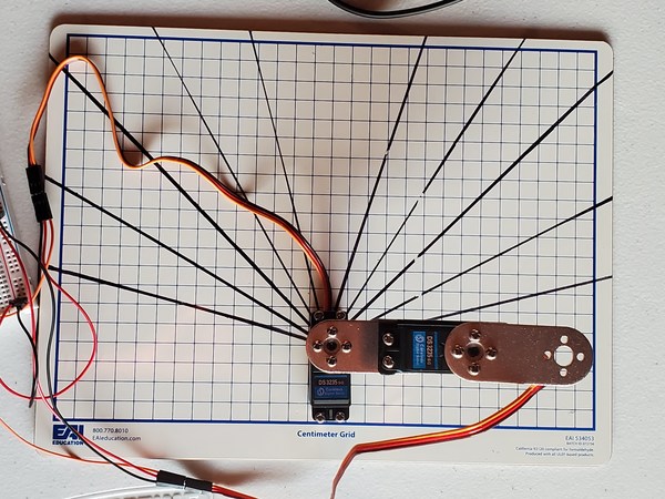
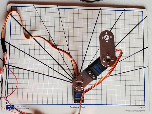
You can try different values for x and y, but make sure those valuables are reachable by the robotic arm. If you input x and y values that are outside the robot’s workspace, your robot will not move at all. It will remain in the home position.
You notice in the code that we used the atan2 function and not atan. Both functions are used to calculate the arctangent. However, unlike atan, atan2 takes into account the signs of both x and y to determine which quadrant the end effector needs to go to.
The returned value for atan is in the range [-90 degrees, 90 degrees], so it only works if your desired end effector coordinate is in Quadrants I or IV of a cartesian grid.
The returned value for atan2 is in the range [-180 degrees, +180 degrees]. It therefore works in all four quadrants of a grid.
atan2 is not as limited as atan, making it useful in our case when we want to make x negative and y positive, for example (which would be in quadrant II of a cartesian grid).
Keep building!
References
Credit to Professor Angela Sodemann from whom I learned these important robotics fundamentals. Dr. Sodemann teaches robotics over at her website, RoboGrok.com. While she uses the PSoC in her work, I use Arduino and Raspberry Pi since I’m more comfortable with these computing platforms. Angela is an excellent teacher and does a fantastic job explaining various robotics topics over on her YouTube channel.

