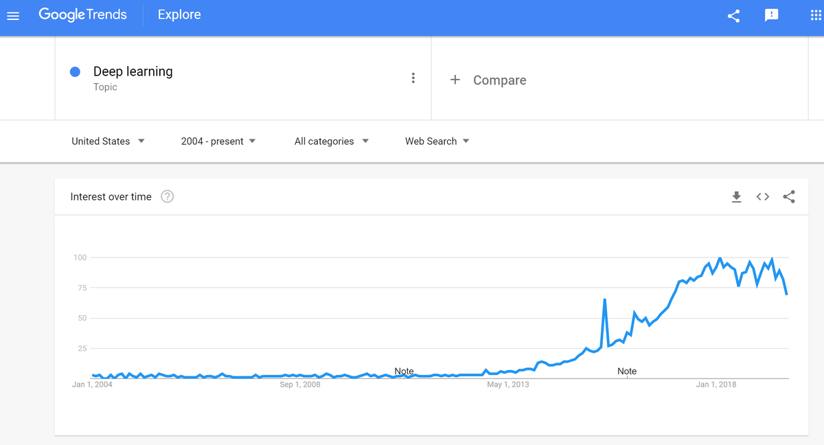
Deep learning has been receiving an enormous amount of interest over the last seven years in the academic and business communities. Let’s take a look at the definition of deep learning, and then we will take a look at how this field has become so popular so quickly.
What is Deep Learning
Deep learning is a machine learning technique in which we teach a computer how to make predictions. Predictions are made by mapping a set of inputs to a set of outputs.
Input Data —–> Deep Learning Algorithm (i.e. Process) —–> Output Data
For example, let’s say our input data into a deep learning algorithm is a set of photos. We want to be able to automatically tag each photo as either being dogs or elephants.


Input Data (lots of images containing dogs and elephants) —–> Deep Learning Algorithm —–> Classification of Each Image (i.e. Dogs or Elephants)
The “learning” part of the term deep learning entails looking at a bunch (hundreds, thousands, even millions+) of photos of elephants and dogs to develop a mathematical model of what both animals look like. Once the deep learning algorithm has been trained to recognize dogs and elephants, it can then be used to classify new photos as either dogs or elephants.
Most deep learning algorithms use neural network architectures as the structure of the underlying mathematical model. For this reason, deep learning methods are commonly called deep neural networks.
Neural networks consist of layers and interconnected nodes. The first layer is the input layer. This layer might consist of, for example, thousands of matrices of pixels that represent photos of dogs or elephants. Each layer after the input layer transforms the data slightly so that the data is more abstract and complete than the previous layer.
The layer after the input layer (i.e. second layer), for example, might contain nodes that recognize simple shapes like circles and edges (that at this point look nothing like a dog or elephant). The third layer contains nodes that recognize more complex shapes that look like a dog’s body parts (e.g. nose, eye, ear, etc.). Then the final layer, the output layer, outputs the classification of a photo as being either a dog or elephant.
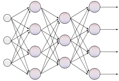
Forbes Magazine has a good image showing the basic deep neural network structure I described above.
The “deep” part of deep learning refers to the number of hidden layers in the neural network. Standard neural networks have two or three (like in my example above) hidden layers, but deep neural networks can have 100+ layers.
In short, a deep neural network is one that has several hidden layers, with the idea that these layers learn different levels of abstraction of the input attributes; thereby allowing the network to solve more complex problems, such as face recognition, object tracking and so on.
Origin of the Deep Learning Revolution: AlexNet
This post at Medium.com shows the graphs of the percentage of selected arXiv publications with either “deep”, “adversarial” or “convolutional” in the title. Note how the graph was virtually all 0s prior to 2010. It then took off like a rocket in 2012. What happened in 2012?
In 2010 and 2011, Fei-Fei Li held the ImageNet competition, an annual machine learning contest. Contest participants were given millions of images to use to train their models. These images were pre-labeled with one of ~1,000 different categories (e.g. leopard, cherry, mushroom, etc.). The objective of the contest was to correctly classify examples that were not in the training set.
During those first two years of the competition in 2010 and 2011, the winning teams had a classification accuracy of 72%. None of the winners of those competitions used deep learning methods. Then in 2012, a team from the University of Toronto led by Alex Krizhevsky won the competition with a classification accuracy of 84%. The second place contestant had a classification accuracy of 74%. The team from the University of Toronto used deep learning methods combined with the computational power of graphical processing units (GPUs) to completely blow the competition out of the water.
The results were remarkable and gave birth to the deep learning era that continues to this day.
Why Deep Learning Has Received So Much Attention Lately
With traditional machine learning approaches, you would have to design a feature extraction algorithm which generally involves a lot of heavy mathematics (complex design), may not be very efficient, and does not perform well (i.e. accuracy may not be suitable for real-world applications). After doing all of that, you would also have to design a whole classification model to classify your input given the extracted features (i.e. attributes).
That’s a lot of work!
Enter Deep Learning…
- With deep neural networks, we can perform feature extraction and classification in one shot, which means we could only need to design one model.
- The availability of large amounts of labeled data as well as GPUs, which can process data in parallel at high speeds, enables these models to be much faster than previous methods.
- Using the back-propagation algorithm, a well-designed loss function, and millions of parameters, these deep networks are able to learn highly complex features (which had to traditionally be hand designed)…i.e. no more complex design!
- Deep neural networks have become fairly easy to implement with high-level open source libraries such as Keras, Pytorch, and TensorFlow.
Deep Learning has made many new applications practically feasible. We wouldn’t have been able to make good language translators pre-deep learning, because we simply had no technique at the time that would perform well enough or at a high enough speed for a real-world application. Deep learning techniques have been applied to not just image recognition, but automatic speech recognition, natural language processing, drug discovery, customer relationship management, robotics, self-driving cars, and more.

