

In this post, I will walk you through the Iterative Dichotomiser 3 (ID3) decision tree algorithm step-by-step. We will develop the code for the algorithm from scratch using Python. We will also run the algorithm on real-world data sets from the UCI Machine Learning Repository.
Table of Contents
- What is the Iterative Dichotomiser 3 Algorithm?
- Iterative Dichotomiser 3 Algorithm Design
- Iterative Dichotomiser 3 Algorithm in Python, Coded From Scratch
- Iterative Dichotomiser 3 Output
What is the Iterative Dichotomiser 3 Algorithm?
Iterative Dichotomiser 3 (ID3)
Unpruned
In the unpruned ID3 algorithm, the decision tree is grown to completion (Quinlan, 1986). The Iterative Dichotomiser 3 (ID3) algorithm is used to create decision trees and was invented by John Ross Quinlan. The decision trees in ID3 are used for classification, and the goal is to create the shallowest decision trees possible.
For example, consider a decision tree to help us determine if we should play tennis or not based on the weather:
- The interior nodes of the tree are the decision variables that are based on the attributes in the data set (e.g. weather outlook [attribute]: sunny, overcast, rainy [attribute values])
- The leaves of the tree store the classifications (e.g. play tennis or don’t play tennis)
Before we get into the details of ID3, let us examine how decision trees work.
How decision trees work
We start with a data set in which each row of the data set corresponds to a single instance. The columns of the data set are the attributes, where the rightmost column is the class label.
Each attribute can take on a set of values. During training of a decision tree, we split the instances in the data set into subsets (i.e. groups) based on the values of the attributes. For example, the weather outlook attribute can be used to create a subset of ‘sunny’ instances, ‘overcast’, and ‘rainy’ instances. We then split each of those subsets even further based on another attribute (e.g. temperature).
The objective behind building a decision tree is to use the attribute values to keep splitting the data into smaller and smaller subsets (recursively) until each subset consists of a single class label (e.g. play tennis or don’t play tennis). We can then classify fresh test instances based on the rules defined by the decision tree.
How ID3 Works
Starting from the root of the tree, ID3 builds the decision tree one interior node at a time where at each node we select the attribute which provides the most information gain if we were to split the instances into subsets based on the values of that attribute. How is “most information” determined? It is determined using the idea of entropy reduction which is part of Shannon’s Information Theory.
Entropy is a measure of the amount of disorder or uncertainty (units of entropy are bits). A data set with a lot of disorder or uncertainty does not provide us a lot of information.
A good way to think about entropy is how certain we would feel if we were to guess the class of a random training instance. A data set in which there is only one class has 0 entropy (high information here because we know with 100% certainty what the class is given an instance). However, if there is a data set in which each instance is a different class, entropy would be high because you have no certainty when trying to predict the class of a random instance.
Entropy is thus a measure of how heterogeneous a data set is. If there are many different class types in a data set, and each class type has the same probability of occurring, the entropy (also impurity) of the data set will be high. The greater the entropy is, the higher the uncertainty, and the less information gained.
Getting back to the running example, in a binary classification problem with positive instances p (play tennis) and negative instances n (don’t play tennis), the entropy contained in a data set is defined mathematically as follows (base 2 log is used as convention in Shannon’s Information Theory).
I(p,n) = entropy of a data set
= weighted sum of the logs of the probabilities of each possible outcome
= -[(p/(p+n))log2(p/(p+n)) + (n/(p+n))log2(n/(p+n))]
= -(p/(p+n))log2(p/(p+n)) + -(n/(p+n))log2(n/(p+n))
Where:
- I = entropy
- p = number of positive instances (e.g. number of play tennis instances)
- n = number of negative instances (e.g. number of don’t play tennis instances)
The negative sign at the beginning of the equation is used to change the negative values returned by the log function to positive values (Kelleher, Namee, & Arcy, 2015). This negation ensures that the logarithmic term returns small numbers for high probabilities (low entropy; greater certainty) and large numbers for small probabilities (higher entropy; less certainty).
Notice that the weights in the summation are the actual probabilities themselves. These weights make sure that classes that appear most frequently in a data set make the biggest impact on the entropy of the data set.
Also notice that if there are only instances with class p (i.e. play tennis) and none with class n (i.e. don’t play tennis) in the data set, the entropy will be 0.
I(p,n) = -(p/(p+n))log2(p/(p+n)) + -(n/(p+n))log2(n/(p+n))
= -(p/(p+0))log2(p/(p+0)) + -(0/(p+0))log2(0/(p+0))
= -(p/p)log2(1) + 0
= 0 + 0
= 0
It is easiest to explain the full ID3 algorithm using actual numbers, so below I will demonstrate how the ID3 algorithm works using an example.
ID3 Example
Continuing from the example in the previous section, we want to create a decision tree that will help us determine if we should play tennis or not.
We have four attributes in our data set:
- Weather outlook: sunny, overcast, rain
- Temperature: hot, mild, cool
- Humidity: high, normal
- Wind: weak, strong
We have two classes:
- p = play tennis class (“Yes”)
- n = don’t play tennis class (“No”)
Here is the data set to train the tree:
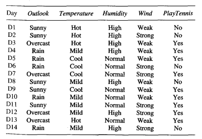
Source: (Mitchell, 1997)
Step 1: Calculate the Prior Entropy of the Data Set
We have 14 total instances: 9 instances of p and 5 instances of n. With the frequency counts of each unique class, we can calculate the prior entropy of this data set where:
- p = number of positive instances (e.g. number of play tennis instances)
- n = number of negative instances (e.g. number of don’t play tennis instances)
Prior Entropy of Data Set = I(p,n)
= weighted sum of the logs of the probabilities of each possible outcome
= -[(p/(p+n))log2(p/(p+n)) + (n/(p+n))log2(n/(p+n))]
= -(p/(p+n))log2(p/(p+n)) + -(n/(p+n))log2(n/(p+n))
= -(9/(9+5))log2(9/(9+5)) + -(5/(9+5))log2(5/(9+5))
= -(9/(9+5))log2(9/(9+5)) + -(5/(9+5))log2(5/(9+5))
= 0.9403
This value above is indicative of how much entropy is remaining prior to doing any splitting.
Step 2: Calculate the Information Gain for Each Attribute
For each attribute in the data set (e.g. outlook, temperature, humidity, and wind):
- Calculate the total number of instances in the data set
- Initialize a running weighted entropy score sum variable to 0.
- Partition the data set instances into subsets based on the attribute values. For example, weather outlook is an attribute. We create the “sunny” subset, “overcast” subset, and “rainy” subset. Therefore, this attribute would create three partitions (or subsets).
- For each attribute value subset:
- Calculate the number of instances in this subset
- Calculate the entropy score of this subset using the frequency counts of each unique class.
- Calculate the weighting of this attribute value by dividing the number of instances in this subset by the total number of instances in the data set
- Add the weighted entropy score for this attribute value to the running weighted entropy score sum.
- The final running weighted entropy score sum is indicative of how much entropy would remain if we were to split the current data set using this attribute. It is the remaining entropy for this attribute.
- Calculate the information gain for this attribute where:
- Information gain = prior entropy of the data set from Step 1 – remaining entropy for this attribute from Step 2
- Record the information gain for this attribute and repeat the process above for the other attributes
For example, consider the first attribute (e.g. weather outlook). The remaining entropy for outlook can be calculated as follows:
Remaining Entropy for Weather Outlook =
= (# of sunny/# of instances)*Isunny(p,n) + (# of overcast/# of instances)*Iovercast(p,n) + (# of rainy/# of instances)*Irainy(p,n)
= (5/14)*Isunny(p,n) + (4/14)*Iovercast(p,n) + (5/14)*Irainy(p,n)
Where:
Isunny(p,n) = I(number of sunny AND Yes, number of sunny AND No)
= I(2,3)
= -(p/(p+n))log2(p/(p+n)) + -(n/(p+n))log2(n/(p+n))
= -(2/(2+3))log2(2/(2+3)) + -(3/(2+3))log2(3/(2+3))
= 0.9710
Iovercast(p,n) = I(number of overcast AND Yes, number of overcast AND No)
= I(4,0)
= -(p/(p+n))log2(p/(p+n)) + -(n/(p+n))log2(n/(p+n))
= -(4/(4+0))log2(4/(4+0)) + -(0/(4+0))log2(0/(4+0))
= 0
Irainy(p,n) = I(number of rainy AND Yes, number of rainy AND No)
= I(3,2)
= -(p/(p+n))log2(p/(p+n)) + -(n/(p+n))log2(n/(p+n))
= -(3/(3+2))log2(3/(3+2)) + -(2/(3+2))log2(2/(3+2))
= 0.9710
Remaining Entropy for Weather Outlook =
= Weighted sum of the entropy scores of each attribute value subset
= (5/14)*Isunny(p,n) + (4/14)*Iovercast(p,n) + (5/14)*Irainy(p,n)
= (5/14) * (0.9710) + (4/14) * 0 + (5/14) * (0.9710)
= 0.6936
Info Gain for Weather Outlook = Prior entropy of the data set – remaining entropy if we split using this attribute
= 0.9403 – 0.6936
= 0.246
Now that we have the information gain for weather outlook, we need to find the remaining entropy and information gain for the other attributes using the same procedure. The remaining entropies for the other attributes are as follows:
- Remaining Entropy for Temperature = 0.911
- Remaining Entropy for Humidity = 0.789
- Remaining Entropy for Wind = 0.892
The information gains are as follows:
- Information Gain for Temperature = 0.9403 – 0.911 = 0.0293
- Information Gain for Humidity = 0.9403 – 0.789 = 0.1513
- Information Gain for Wind = 0.9403 – 0.892 = 0.0483
Step 3: Calculate the Attribute that Had the Maximum Information Gain
The information gain for weather outlook is 0.246, so it provides the most information and becomes the label for the root node.
Step 4: Partition the Data Set Based on the Values of the Attribute that Had the Maximum Information Gain
The data set is then partitioned based on the values this maximum information gain attribute can take (e.g. sunny, overcast, and rain). The partitions become the outgoing branches from the root node. These branches terminate in new unlabeled nodes. The maximum information gain attribute is removed from these partitions and is not used again to make any more splits from these new unlabeled nodes. An attribute can only be used as a decision variable once on a given path in a tree but can be used multiple times in an entire tree.
Step 5: Repeat Steps 1-4 for Each Branch of the Tree Using the Relevant Partition
We stop when:
- Every instance in the partition is part of the same class. Return a decision tree that is made up of a leaf node and labeled with the class of the instances.
- There are no more attributes left. Return a decision tree that is made up of a leaf node labeled with the class that comprised the majority of the instances.
- No instances in the partition. We return a decision tree that is made up of a leaf node and label with the most common class in the parent node.
Here is the final decision tree:
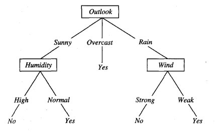
Source: (Mitchell, 1997)
Information Gain Ratio
An issue with just using information gain as the selection criteria for the root is that it has a strong bias towards selecting attributes that contain a large number of different values (which could lead to trees that overfit to the data). One way to rectify this is to use what is called the gain ratio. It acts as a kind of normalization factor.
The gain ratio defines an additional term that penalizes attributes that create a large number of partitions. The gain ratio chooses attributes based on the ratio between their gain and their intrinsic information content. It represents the proportion of information generated that is useful for classification. The attribute with the highest gain ratio is selected as the attribute that splits the data at that node.
Gain Ratio of an Attribution = Information Gain of the Attribute / Split Information of the Attribute
The clearest way to demonstrate the information gain is to show an example. Going back to our original data set, suppose we partition the data set based on the outlook attribute. This partition will result in three subsets: “sunny” subset (frequency count of 5), “overcast” subset (frequency count of 4), and “rainy” subset (frequency count of 5).
Split Information of Outlook = -[(5/14) * log2(5/14) + (4/14) * log2(4/14) + (5/14) * log2(5/14)] = 1.577
The gain was calculated as 0.246, so the gain ratio is 0.246 / 1.577 = 0.156.
For humidity, we can also calculate the gain ratio.
Split Information of Humidity = -[(7/14) * log2(7/14) + (7/14) * log2(7/14)] = 1
The gain was calculated as 0.1513, so the gain ratio is 0.1513 / 1 = 0.1513.
Pruned
One common way to resolve the issue of overfitting is to do reduced error pruning (Mitchell, 1997).
- Training, validation, and test sets are used.
- A portion of the original data set is withheld as a validation set. This validation set is not used during the training phase of the tree (i.e. while the decision tree is getting built).
- Once training is finished and the decision tree is built, the tree is tested on the validation set.
- Each node is considered as a candidate for pruning. Pruning means removing the subtree at that node, making it a leaf, and assigning the most common class at the node.
- A node is removed if the resulting pruned tree has a classification accuracy (as tested against the validation set) that is at least as good as the accuracy of the original decision tree.
- If replacing the subtree by a leaf results in improved classification accuracy, replace the subtree with that leaf.
- Pruning continues until no further improvement in the classification accuracy occurs.
- This process happens in a depth-first manner, starting from the leaves.
Iterative Dichotomiser 3 Algorithm Design
The ID3 algorithm was implemented from scratch with and without reduced error pruning. The abalone, car evaluation, and image segmentation data sets were then preprocessed to meet the input requirements of the algorithms.
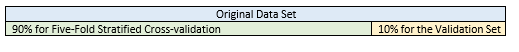
Five-Fold Cross-Validation
In this project, for the pruned version of ID3, 10% of the data was pulled out of the original data set to be used as a validation set. The remaining 90% of the data was used for five-fold stratified cross-validation to evaluate the performance of the models. For the unpruned version, the entire data set was used for five-fold stratified cross-validation.
Required Data Set Format for ID3
Required Data Set Format for ID3-Unpruned
- Columns (0 through N)
- 0: Class
- 1: Attribute 1
- 2: Attribute 2
- 3: Attribute 3
- N: Attribute N
Required Data Set Format for ID3-Pruned
- Columns (0 through N)
- 0: Class
- 1: Attribute 1
- 2: Attribute 2
- 3: Attribute 3
- N: Attribute N
Abalone Data Set
The original abalone data set contains 4177 instances, 8 attributes, and 29 classes (Waugh, 1995). The purpose of this data set is to predict the age of an abalone from physical measurements.
Modification of Attribute Values
All attribute values except for the sex attribute were made discrete by putting the continuous values into bins based on the quartile the value fell into. This modification follows the principle of Occam’s Razor.
Some of the classes only had one or two instances, so the class values (ages of the abalones) were converted into three classes of approximately equal size:
- Young = 0
- Middle-Aged = 1
- Old = 2
Missing Data
There were no missing attribute values.
Car Evaluation Data Set
The original car evaluation data set contains 6 attributes and 1728 instances (Bohanec, 1997). The purpose of the data set is to predict car acceptability based on price, comfort, and technical specifications.
Modification of Attribute Values
No modification of attribute values was necessary since all attributes were discrete.
Missing Data
There were no missing attribute values.
Image Segmentation Data Set
This data set is used for classification. It contains 19 attributes, 210 instances, and 7 classes (Brodley, 1990). This data set was created from a database of seven outdoor images.
Modification of Attribute Values
All attribute values were made discrete by putting the continuous values into bins based on the quartile the value fell into.
The class values were already discrete and were left as-is.
Missing Data
There were no missing attribute values.
Iterative Dichotomiser 3 Algorithm in Python, Coded From Scratch
Here are the preprocessed data sets:
Here is the code that parses the input file. Don’t be scared at how long all this code is. I include a lot of comments so that you know what is going on (just copy and paste all these programs into your favorite IDE, and you are good to go!):
import csv # Library to handle csv-formatted files

# File name: parse.py
# Author: Addison Sears-Collins
# Date created: 7/6/2019
# Python version: 3.7
# Description: Used for parsing the input data file

def parse(filename):
    """
    Parameters:
        filename: Name of a file
    Returns:
        data: Information on the attributes and the data as a list of
              dictionaries. Each instance is a different dictionary.
    """

    # Initialize an empty list named 'data'
    data = []

    # Open the file in READ mode.
    # The file object is named 'file'
    with open(filename, 'r') as file:

        # Convert the file object named file to a csv.reader object. Save the
        # csv.reader object as csv_file
        csv_file = csv.reader(file)

        # Return the current row (first row) and advance the iterator to the
        # next row. Since the first row contains the attribute names (headers),
        # save them in a list called headers
        headers = next(csv_file)

        # Extract each of the remaining data rows one row at a time
        for row in csv_file:
            # append method appends an element to the end of the list
            # The element that is appended is a dictionary.
            # A dictionary contains search key-value pairs, analogous to
            # word-definition in a regular dictionary.
            # In this case, each instance is a separate dictionary.
            # The zip method joins two lists together so that we have
            # attributename(header)-value(row) pairs for each instance
            # in the data set
            data.append(dict(zip(headers, row)))

    return data

##Used for debugging
#name_of_file =  "abalone.txt"
#data = parse(name_of_file)
#print(*data, sep = "\n")
#print()
#print(str(len(data)))
Here is the code for five-fold stratified cross-validation:
import random
from collections import Counter # Used for counting

# File name: five_fold_stratified_cv.py
# Author: Addison Sears-Collins
# Date created: 7/7/2019
# Python version: 3.7
# Description: Implementation of five-fold stratified cross-validation
# Divide the data set into five random groups. Make sure
# that the proportion of each class in each group is roughly equal to its
# proportion in the entire data set.

# Required Data Set Format for Classification Problems:
# Columns (0 through N)
# 0: Class
# 1: Attribute 1
# 2: Attribute 2
# 3: Attribute 3
# ...
# N: Attribute N

def get_five_folds(instances):
    """
    Parameters:
        instances: A list of dictionaries where each dictionary is an instance.
            Each dictionary contains attribute:value pairs
    Returns:
        fold0, fold1, fold2, fold3, fold4
        Five folds whose class frequency distributions are
        each representative of the entire original data set (i.e. Five-Fold
        Stratified Cross Validation)
    """
    # Create five empty folds
    fold0 = []
    fold1 = []
    fold2 = []
    fold3 = []
    fold4 = []

    # Shuffle the data randomly
    random.shuffle(instances)

    # Generate a list of the unique class values and their counts
    classes = []  # Create an empty list named 'classes'

    # For each instance in the list of instances, append the value of the class
    # to the end of the classes list
    for instance in instances:
        classes.append(instance['Class'])

    # Create a list of the unique classes
    unique_classes = list(Counter(classes).keys())

    # For each unique class in the unique class list
    for uniqueclass in unique_classes:

        # Initialize the counter to 0
        counter = 0

        # Go through each instance of the data set and find instances that
        # are part of this unique class. Distribute them among one
        # of five folds
        for instance in instances:

            # If we have a match
            if uniqueclass == instance['Class']:

                # Allocate instance to fold0
                if counter == 0:

                    # Append this instance to the fold
                    fold0.append(instance)

                    # Increase the counter by 1
                    counter += 1

                # Allocate instance to fold1
                elif counter == 1:

                    # Append this instance to the fold
                    fold1.append(instance)

                    # Increase the counter by 1
                    counter += 1

                # Allocate instance to fold2
                elif counter == 2:

                    # Append this instance to the fold
                    fold2.append(instance)

                    # Increase the counter by 1
                    counter += 1

                # Allocate instance to fold3
                elif counter == 3:

                    # Append this instance to the fold
                    fold3.append(instance)

                    # Increase the counter by 1
                    counter += 1

                # Allocate instance to fold4
                else:

                    # Append this instance to the fold
                    fold4.append(instance)

                    # Reset the counter to 0
                    counter = 0

    # Shuffle the folds
    random.shuffle(fold0)
    random.shuffle(fold1)
    random.shuffle(fold2)
    random.shuffle(fold3)
    random.shuffle(fold4)

    # Return the folds
    return  fold0, fold1, fold2, fold3, fold4
Here is the ID3 code:
from node import Node # Import the Node class from the node.py file
from math import log # We need this to compute log base 2
from collections import Counter # Used for counting

# File name: id3.py
# Author: Addison Sears-Collins
# Date created: 7/5/2019
# Python version: 3.7
# Description: Iterative Dichotomiser 3 algorithm

# Required Data Set Format for Classification Problems:
# Columns (0 through N)
# 0: Class
# 1: Attribute 1
# 2: Attribute 2
# 3: Attribute 3
# ...
# N: Attribute N

def ID3(instances, default):
    """
    Parameters:
      instances: A list of dictionaries where each dictionary is an instance.
                 Each dictionary contains attribute:value pairs
                 e.g.: instances =
                   {'Class':'Play','Outlook':'Sunny','Temperature':'Hot'}
                   {'Class':'Don't Play','Outlook':'Rain','Temperature':'Cold'}
                   {'Class':'Play','Outlook':'Overcast','Temperature':'Hot'}
                   ...
                   etc.
                 The first attribute:value pair is the
                 target variable (i.e. the class of that instance)
      default: The default class label (e.g. 'Play')
    Returns:
      tree: An object of the Node class
    """
    # The len method returns the number of items in the list
    # If there are no more instances left, return a leaf that is labeled with
    # the default class
    if len(instances) == 0:
        return Node(default)

    classes = []  # Create an empty list named 'classes'

    # For each instance in the list of instances, append the value of the class
    # to the end of the classes list
    for instance in instances:
        classes.append(instance['Class'])

    # If all instances have the same class label or there is only one instance
    # remaining, create a leaf node labeled with that class.
    # Counter(list) creates a tally of each element in the list. This tally is
    # represented as an element:tally pair.
    if len(Counter(classes)) == 1 or len(classes) == 1:
        tree = Node(mode_class(instances))
        return tree

    # Otherwise, find the best attribute, the attribute that maximizes the gain
    # ratio of the data set, to be the next decision node.
    else:
        # Find the name of the most informative attribute of the data set
        # e.g. "Outlook"
        best_attribute = most_informative_attribute(instances)

        # Initialize a tree with the most common class
        # e.g. "Play"
        tree = Node(mode_class(instances))

        # The most informative attribute becomes this decision node
        # e.g. "Outlook" becomes this node
        tree.attribute = best_attribute

        best_attribute_values = []

        # The branches of the node are the values of the best_attribute
        # e.g. "Sunny", "Overcast", "Rainy"
        # Go through each instance and create a list of the values of
        # best_attribute
        for instance in instances:
            try:
                best_attribute_values.append(instance[best_attribute])
            except:
                no_best_attribute = True
        # Create a list of the unique best attribute values
        # Set is like a list except it extracts nonduplicate (unique)
        # items from a list.
        # In short, we create a list of the set of unique
        # best attribute values.
        tree.attribute_values = list(set(best_attribute_values))

        # Now we need to split the instances. We will create separate subsets
        # for each best attribute value. These become the child nodes
        # i.e. "Sunny", "Overcast", "Rainy" subsets
        for best_attr_value_i in tree.attribute_values:

            # Generate the subset of instances
            instances_i = []
            # Go through one instance at a time
            for instance in instances:
                # e.g. If this instance has "Sunny" as its best attribute value
                if instance[best_attribute] == best_attr_value_i:
                    instances_i.append(instance) #Add this instance to the list

            # Create a subtree recursively
            subtree = ID3(instances_i, mode_class(instances))

            # Initialize the values of the subtree
            subtree.instances_labeled = instances_i

            # Keep track of the state of the subtree's parent (i.e. tree)
            subtree.parent_attribute = best_attribute # parent node
            subtree.parent_attribute_value = best_attr_value_i # branch name

            # Assign the subtree to the appropriate branch
            tree.children[best_attr_value_i] = subtree

        # Return the decision tree
        return tree


def mode_class(instances):
    """
    Parameters:
      instances: A list of dictionaries where each dictionary is an instance.
        Each dictionary contains attribute:value pairs
    Returns:
      Name of the most common class (e.g. 'Don't Play')
    """

    classes = []  # Create an empty list named 'classes'

    # For each instance in the list of instances, append the value of the class
    # to the end of the classes list
    for instance in instances:
        classes.append(instance['Class'])

    # The 1 ensures that we get the top most common class
    # The [0][0] ensures we get the name of the class label and not the tally
    # Return the name of the most common class of the instances
    return Counter(classes).most_common(1)[0][0]

def prior_entropy(instances):
    """
    Calculate the entropy of the data set with respect to the actual class
    prior to splitting the data.
    Parameters:
      instances: A list of dictionaries where each dictionary is an instance.
        Each dictionary contains attribute:value pairs
    Returns:
      Entropy value in bits
    """
    # For each instance in the list of instances, append the value of the class
    # to the end of the classes list
    classes = []  # Create an empty list named 'classes'

    for instance in instances:
        classes.append(instance['Class'])
    counter = Counter(classes)

    # If all instances have the same class, the entropy is 0
    if len(counter) == 1:
        return 0
    else:
    # Compute the weighted sum of the logs of the probabilities of each
    # possible outcome
        entropy = 0
        for c, count_of_c in counter.items():
            probability = count_of_c / len(classes)
            entropy += probability * (log(probability, 2))
        return -entropy

def entropy(instances, attribute, attribute_value):
    """
    Calculate the entropy for a subset of the data filtered by attribute value
    Parameters:
      instances: A list of dictionaries where each dictionary is an instance.
        Each dictionary contains attribute:value pairs
      attribute: The name of the attribute (e.g. 'Outlook')
      attribute_value: The value of the attribute (e.g. 'Sunny')
    Returns:
      Entropy value in bits
    """
    # For each instance in the list of instances, append the value of the class
    # to the end of the classes list
    classes = []  # Create an empty list named 'classes'

    for instance in instances:
        if instance[attribute] == attribute_value:
            classes.append(instance['Class'])
    counter = Counter(classes)

    # If all instances have the same class, the entropy is 0
    if len(counter) == 1:
        return 0
    else:
    # Compute the weighted sum of the logs of the probabilities of each
    # possible outcome
        entropy = 0
        for c, count_of_c in counter.items():
            probability = count_of_c / len(classes)
            entropy += probability * (log(probability, 2))
        return -entropy

def gain_ratio(instances, attribute):
    """
    Calculate the gain ratio if we were to split the data set based on the values
    of this attribute.
    Parameters:
      instances: A list of dictionaries where each dictionary is an instance.
        Each dictionary contains attribute:value pairs
      attribute: The name of the attribute (e.g. 'Outlook')
    Returns:
      The gain ratio
    """
    # Record the entropy of the combined set of instances
    priorentropy = prior_entropy(instances)

    values = []

    # Create a list of the attribute values for each instance
    for instance in instances:
        values.append(instance[attribute])
    counter = Counter(values) # Store the frequency counts of each attribute value

    # The remaining entropy if we were to split the instances based on this attribute
    # This is a weighted entropy score sum
    remaining_entropy = 0

    # This variable is used for the gain ratio calculation
    split_information = 0

    # items() method returns a list of all dictionary key-value pairs
    for attribute_value, attribute_value_count in counter.items():
        probability = attribute_value_count/len(values)
        remaining_entropy += (probability * entropy(
            instances, attribute, attribute_value))
        split_information += probability * (log(probability, 2))

    information_gain = priorentropy - remaining_entropy

    split_information = -split_information

    gainratio = None

    if split_information != 0:
        gainratio = information_gain / split_information
    else:
        gainratio = -1000

    return gainratio

def most_informative_attribute(instances):
    """
    Choose the attribute that provides the most information if you were to
    split the data set based on that attribute's values. This attribute is the
    one that has the highest gain ratio.
    Parameters:
      instances: A list of dictionaries where each dictionary is an instance.
        Each dictionary contains attribute:value pairs
      attribute: The name of the attribute (e.g. 'Outlook')
    Returns:
      The name of the most informative attribute
    """
    selected_attribute = None
    max_gain_ratio = -1000

    # instances[0].items() extracts the first instance in instances
    # for key, value iterates through each key-value pair in the first
    # instance in instances
    # In short, this code creates a list of the attribute names
    attributes = [key for key, value in instances[0].items()]
    # Remove the "Class" attribute name from the list
    attributes.remove('Class')

    # For every attribute in the list of attributes
    for attribute in attributes:
        # Calculate the gain ratio and store that value
        gain = gain_ratio(instances, attribute)

        # If we have a new most informative attribute
        if gain > max_gain_ratio:
            max_gain_ratio = gain
            selected_attribute = attribute

    return selected_attribute

def accuracy(trained_tree, test_instances):
    """
    Parameters:
        trained_tree: A tree that has already been trained
        test_instances: A set of test instances
    Returns:
        Classification accuracy (# of correct predictions/# of predictions)
    """
    # Set the counter to 0
    no_of_correct_predictions = 0

    for test_instance in test_instances:
        if predict(trained_tree, test_instance) == test_instance['Class']:
            no_of_correct_predictions += 1

    return no_of_correct_predictions / len(test_instances)

def predict(node, test_instance):
    '''
    Parameters:
        node: A trained tree node
        test_instance: A single test instance
    Returns:
        Class value (e.g. "Play")
    '''
    # Stopping case for the recursive call.
    # If this is a leaf node (i.e. has no children)
    if len(node.children) == 0:
        return node.label
    # Otherwise, we are not yet on a leaf node.
    # Call predict method recursively until we get to a leaf node.
    else:
        # Extract the attribute name (e.g. "Outlook") from the node.
        # Record the value of the attribute for this test instance into
        # attribute_value (e.g. "Sunny")
        attribute_value = test_instance[node.attribute]

        # Follow the branch for this attribute value assuming we have
        # an unpruned tree.
        if attribute_value in node.children and node.children[
            attribute_value].pruned == False:
            # Recursive call
            return predict(node.children[attribute_value], test_instance)

        # Otherwise, return the most common class
        # return the mode label of examples with other attribute values for the current attribute
        else:
            instances = []
            for attr_value in node.attribute_values:
                instances += node.children[attr_value].instances_labeled
            return mode_class(instances)

TREE = None
def prune(node, val_instances):
    """
    Prune the tree recursively, starting from the leaves
    Parameters:
        node: A tree that has already been trained
        val_instances: The validation set
    """
    global TREE
    TREE = node

    def prune_node(node, val_instances):
        # If this is a leaf node
        if len(node.children) == 0:
            accuracy_before_pruning = accuracy(TREE, val_instances)
            node.pruned = True

            # If no improvement in accuracy, no pruning
            if accuracy_before_pruning >= accuracy(TREE, val_instances):
                node.pruned = False
            return

        for value, child_node in node.children.items():
            prune_node(child_node, val_instances)

        # Prune when we reach the end of the recursion
        accuracy_before_pruning = accuracy(TREE, val_instances)
        node.pruned = True

        if accuracy_before_pruning >= accuracy(TREE, val_instances):
            node.pruned = False

    prune_node(TREE, val_instances)
Here is the code for the nodes. This is needed in order to run ID3 (above).
# File name: node.py
# Author: Addison Sears-Collins
# Date created: 7/6/2019
# Python version: 3.7
# Description: Used for constructing nodes for a tree

class Node:

  # Method used to initialize a new node's data fields with initial values
  def __init__(self, label):

    # Declaring variables specific to this node
    self.attribute = None  # Attribute (e.g. 'Outlook')
    self.attribute_values = []  # Values (e.g. 'Sunny')
    self.label = label   # Class label for the node (e.g. 'Play')
    self.children = {}   # Keeps track of the node's children

    # References to the parent node
    self.parent_attribute = None
    self.parent_attribute_value = None

    # Used for pruned trees
    self.pruned = False  # Is this tree pruned?
    self.instances_labeled = []
Here is the code that displays the results. This is the driver program:
import id3
import parse
import random
import five_fold_stratified_cv
from matplotlib import pyplot as plt


# File name: results.py
# Author: Addison Sears-Collins
# Date created: 7/6/2019
# Python version: 3.7
# Description: Results of the Iterative Dichotomiser 3 runs
# This source code is the driver for the entire program

# Required Data Set Format for Classification Problems:
# Columns (0 through N)
# 0: Class
# 1: Attribute 1
# 2: Attribute 2
# 3: Attribute 3
# ...
# N: Attribute N

ALGORITHM_NAME = "Iterative Dichotomiser 3"

def main():

    print("Welcome to the " +  ALGORITHM_NAME + " Program!")
    print()

    # Enter the name of your input file
    #file_name = 'car.txt'
    file_name = input("Enter the name of your input file (e.g. car.txt): ")


    # Show functioning of the program
    #trace_runs_file = 'car_id3_trace_runs.txt'
    trace_runs_file = input(
       "Enter the name of your trace runs file (e.g. car_id3_trace_runs.txt): ")

    # Save the output graph of the results
    #imagefile = 'car_id3_results.png'
    imagefile = input(
        "Enter the name of the graphed results file (e.g. foo.png): ")

    # Open a new file to save trace runs
    outfile_tr = open(trace_runs_file,"w")

    outfile_tr.write("Welcome to the " +  ALGORITHM_NAME + " Program!" + "\n")
    outfile_tr.write("\n")

    data = parse.parse(file_name)
    pruned_accuracies_avgs = []
    unpruned_accuracies_avgs = []

    # Shuffle the data randomly
    random.shuffle(data)

    # This variable is used for the final graph. Places
    # upper limit on the x-axis.
    # 10% of is pulled out for the validation set
    # 20% of that set is used for testing in the five-fold
    # stratified cross-validation
    # Round up to the nearest value of 10
    upper_limit = (round(len(data) * 0.9 * 0.8) - round(
        len(data) * 0.9 * 0.8) % 10) + 10
    #print(str(upper_limit)) # Use for debugging
    if upper_limit <= 10:
        upper_limit = 50

    # Get the most common class in the data set.
    default = id3.mode_class(data)

    # Pull out 10% of the data to be used as a validation set
    # The remaining 90% of the data is used for cross validation.
    validation_set = data[: 1*len(data)//10]
    data = data[1*len(data)//10 : len(data)]

    # Generate the five stratified folds
    fold0, fold1, fold2, fold3, fold4 = five_fold_stratified_cv.get_five_folds(
        data)

    # Generate lists to hold the training and test sets for each experiment
    testset = []
    trainset = []

    # Create the training and test sets for each experiment
    # Experiment 0
    testset.append(fold0)
    trainset.append(fold1 + fold2 + fold3 + fold4)

    # Experiment 1
    testset.append(fold1)
    trainset.append(fold0 + fold2 + fold3 + fold4)

    # Experiment 2
    testset.append(fold2)
    trainset.append(fold0 + fold1 + fold3 + fold4)

    # Experiment 3
    testset.append(fold3)
    trainset.append(fold0 + fold1 + fold2 + fold4)

    # Experiment 4
    testset.append(fold4)
    trainset.append(fold0 + fold1 + fold2 + fold3)

    step_size = len(trainset[0])//20

    for length in range(10, upper_limit, step_size):
        print('Number of Training Instances:', length)
        outfile_tr.write('Number of Training Instances:' + str(length) +"\n")
        pruned_accuracies = []
        unpruned_accuracies = []

        # Run all 5 experiments for 5-fold stratified cross-validation
        for experiment in range(5):

            # Each experiment has a training and testing set that have been
            # preassigned.
            train = trainset[experiment][: length]
            test = testset[experiment]

            # Pruned
            tree = id3.ID3(train, default)
            id3.prune(tree, validation_set)
            acc = id3.accuracy(tree, test)
            pruned_accuracies.append(acc)

            # Unpruned
            tree = id3.ID3(train, default)
            acc = id3.accuracy(tree, test)
            unpruned_accuracies.append(acc)

        # Calculate and store the average classification
        # accuracies for each experiment
        avg_pruned_accuracies = sum(pruned_accuracies) / len(pruned_accuracies)
        avg_unpruned_accuracies = sum(unpruned_accuracies) / len(unpruned_accuracies)

        print("Classification Accuracy for Pruned Tree:", avg_pruned_accuracies)
        print("Classification Accuracy for Unpruned Tree:", avg_unpruned_accuracies)
        print()
        outfile_tr.write("Classification Accuracy for Pruned Tree:" + str(
            avg_pruned_accuracies) + "\n")
        outfile_tr.write("Classification Accuracy for Unpruned Tree:" + str(
                avg_unpruned_accuracies) +"\n\n")

        # Record the accuracies, so we can plot them later
        pruned_accuracies_avgs.append(avg_pruned_accuracies)
        unpruned_accuracies_avgs.append(avg_unpruned_accuracies)

    # Close the file
    outfile_tr.close()

    plt.plot(range(10, upper_limit, step_size), pruned_accuracies_avgs, label='pruned tree')
    plt.plot(range(10, upper_limit, step_size), unpruned_accuracies_avgs, label='unpruned tree')
    plt.xlabel('Number of Training Instances')
    plt.ylabel('Classification Accuracy on Test Instances')
    plt.grid(True)
    plt.title("Learning Curve for " +  str(file_name))
    plt.legend()
    plt.savefig(imagefile)
    plt.show()


main()
Iterative Dichotomiser 3 Output
Here are the trace runs:
Here are the results:
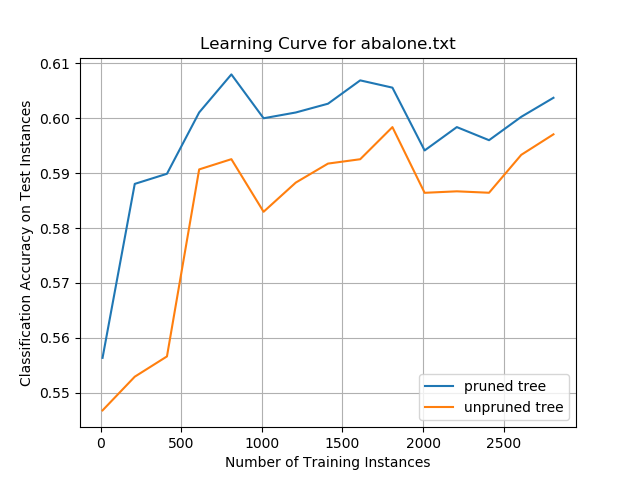
Abalone Data Set
Car Evaluation Data Set
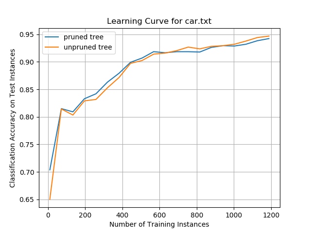
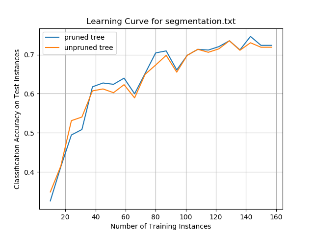
Image Segmentation Data Set
Analysis
Abalone Data Set
While the overall classification accuracies on the data set were only ~60%, the data show the impact that pruning a decision tree can have on improving prediction performance. The pruned tree performed better than the unpruned tree on the same set of test instances, irrespective of how many training instances the decision trees were trained on. These results suggest that smaller decision trees can generalize better than larger trees and can more accurately classify new test instances. This pruning impact was more pronounced on this data set than any of the other data sets evaluated in this project.
Car Evaluation Data Set
Classification accuracy for both the pruned and unpruned trees was high on this data set, plateauing at ~92%. This performance was the best of any of the data sets examined in this project.
When the decision trees were trained on a relatively small number of training instances, the pruned trees outperformed the unpruned trees. However, beyond 600 training instances, unpruned trees began to have higher classification accuracy.
It is not clear if the superior accuracy of the unpruned tree algorithm on large numbers of training instances was due to overfitting on the training data or if there was actually an improvement in performance. More training data would be needed to examine if this effect remains consistent for larger numbers of training instances.
Image Segmentation Data Set
For the segmentation data set, neither the unpruned nor the pruned trees outperformed the other consistently. Overall classification accuracy quickly improved for both ID3 algorithms when the decision trees were trained on more training instances. Performance plateaued at ~72%, which was not as good as the car evaluation data set but was better than the abalone data set.
The results show that creating smaller decision trees by pruning the branches might not lead to improved classification performance on unseen new test instances, in some cases.
Summary and Conclusions
We can conclude that decision trees can create a convenient set of if-then-else decision rules that can be used to classify new unseen test instances. Classification accuracy for both the pruned and unpruned ID3 algorithms was >60% for all data sets, reaching a peak of ~92% on the car evaluation data set.
Neither type of tree, unpruned and pruned, consistently outperformed the other in terms of classification accuracy. The results suggest the impact of pruning depends highly on the data set being evaluated. On the abalone data set, pruning the tree reduced overfitting and led to improved performance. On the car evaluation data set, the performance was mixed. On the image segmentation data set, performance was relatively the same for both ID3-unpruned and ID3-pruned.
In a real-world setting, the overhead associated with reduced error pruning would need to be balanced against the increased speed and simplicity with which new unseen test instances could be classified. Future work would need to compare the performance of the ID3-pruned and ID3-unpruned algorithms on other classification data sets.
References
Alpaydin, E. (2014). Introduction to Machine Learning. Cambridge, Massachusetts: The MIT Press.
Bohanec, M. (1997, 6 1). Car Evaluation Data Set. Retrieved from UCI Machine Learning Repository: https://archive.ics.uci.edu/ml/datasets/Car+Evaluation
Brodley, C. (1990, November 1). Image Segmentation Data Set. Retrieved from UCI Machine Learning Repository: https://archive.ics.uci.edu/ml/datasets/Image+Segmentation
James, G. (2013). An Introduction to Statistical Learning: With Applications in R. New York: Springer.
Kelleher, J. D., Namee, B., & Arcy, A. (2015). Fundamentals of Machine Learning for Predictive Data Analytics. Cambridge, Massachusetts: The MIT Press.
Mitchell, T. M. (1997). Machine Learning. New York: McGraw-Hill.
Quinlan, J. R. (1986). Induction of Decision Trees. Machine Learning, 81-106.
Waugh, S. (1995, 12 1). Abalone Data Set. Retrieved from UCI Machine Learning Repository: https://archive.ics.uci.edu/ml/datasets/Abalone