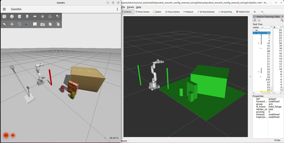
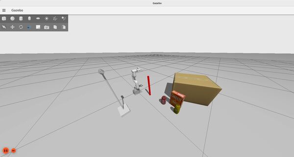
In this tutorial, we’ll enhance our previous pick and place application by incorporating visual perception. We will still use the MoveIt Task Constructor for ROS 2. Here is what you will build by the end of this tutorial:

Building upon our earlier work, we’ll now use a depth camera to dynamically detect and locate objects in the scene, replacing the need for hardcoded object positions. This advancement will make our pick and place operation more flexible, robust, and adaptable to real-world scenarios.

We’ll modify our existing application to show how visual input can be integrated with the MoveIt Task Constructor framework. By the end of this tutorial, you’ll have created a vision-enhanced pick and place system that demonstrates the power of combining perception with sophisticated motion planning.

Here is what skills you will learn in this tutorial:

1. Learn how to integrate a simulated depth camera into Gazebo
2. Learn how to process point cloud data to detect and locate objects.
   • A point cloud is a collection of data points in 3D space that represent the surface of an object or environment.
3. Learn how to dynamically update the MoveIt planning scene based on visual information
4. Learn how to modify the MoveIt Task Constructor pipeline to use real-time object poses (positions and orientations)

Here is a high-level overview of what our enhanced program will do:

1. Set up the demo scene with randomly placed objects
2. Acquire and process point cloud data from the depth camera
3. Detect and localize objects in the scene
4. Update the planning scene with the detected objects
5. Define a pick sequence that includes:
   • Opening the gripper
   • Moving to a visually determined pre-grasp position
   • Approaching the target object
   • Closing the gripper
   • Lifting the object
6. Define a place sequence that includes:
   • Moving to a designated place location
   • Lowering the object
   • Opening the gripper
   • Retreating from the placed object
7. Plan the entire pick and place task using the updated scene information
8. Optionally execute the planned task
9. Provide detailed feedback on each stage of the process, including visual perception results

Real-World Use Cases

Same real-world use cases as in the previous tutorial.

Prerequisites

• You have completed this tutorial.

All the code is here on my GitHub repository. Note that I am working with ROS 2 Iron, so the steps might be slightly different for other versions of ROS 2.

Install Cyclone DDS

First we need to install Cyclone DDS, and make it the default middleware to enable the different nodes to communicate with each other with low latency. You don’t need to understand how Cyclone DDS works.

Open a terminal window, and type:

sudo apt install ros-$ROS_DISTRO-rmw-cyclonedds-cpp

echo '# MoveIt recommends CycloneDDS as a middleware (Source: https://moveit.ai/install-moveit2/binary/)' >> ~/.bashrc

echo 'export RMW_IMPLEMENTATION=rmw_cyclonedds_cpp' >> ~/.bashrc

Install the PCL-ROS Package

Later on in this tutorial, to see point cloud (.pcd) files in RViz2, you will need the PCL-ROS package.

sudo apt-get install ros-$ROS_DISTRO-pcl-ros

Create a Package

Let’s create a package to store our code.

cd ~/ros2_ws/src/mycobot_ros2/

ros2 pkg create --build-type ament_cmake --dependencies moveit_core moveit_ros_planning_interface moveit_task_constructor_core rclcpp --license BSD-3-Clause hello_mtc_with_perception

Create a Launch File 

Now let’s create some launch files. Here are all the launch files.

cd ~/ros2_ws/src/mycobot_ros2/hello_mtc_with_perception/

Create a folder named launch.

mkdir launch

cd launch

Add your first launch file: 

gedit run.launch.py 

This launch file sets up MoveIt 2 for the myCobot robotic arm. It configures various paths, sets up MoveIt with settings for trajectory execution, kinematics, and planning pipelines, and launches the move_group node for motion planning. It also optionally starts RViz for visualization.

Save the file, and close it. 

gedit demo.launch.py 

This launch file is designed for running a demo of the MoveIt Task Constructor with perception capabilities. It sets up the necessary configurations, launches the required nodes, and provides parameters for the demo execution, including robot description, kinematics, and planning pipelines.

Save the file, and close it. 

gedit robot.launch.py 

This launch file is responsible for launching the robotic arm in the Gazebo simulation environment. It sets up the Gazebo world, starts the robot state publisher, initializes various controllers for the arm and gripper, and spawns the robot model.

Save the file, and close it. 

gedit point_cloud_viewer.launch.py 

This launch file is created for viewing point cloud data (.pcd files) in RViz. It starts a node to convert PCD files to point clouds, allows configuration of file paths and publishing intervals, and launches RViz with a specific configuration for visualizing the point cloud data.

Save the file, and close it. 

gedit get_planning_scene_server.launch.py 

This launch file starts the GetPlanningSceneServer node (we’ll go over this service in detail later in this tutorial), which is responsible for providing the current planning scene. It loads configuration parameters from a YAML file.

Save the file, and close it.

Create a Parameter File

Now let’s add some parameters.

cd ~/ros2_ws/src/mycobot_ros2/hello_mtc_with_perception/

mkdir config

cd config

gedit mtc_node_params.yaml 

This YAML file contains configuration parameters for the MoveIt Task Constructor node. It includes settings for robot control, object manipulation, motion planning, and various timeout and scaling factors. These parameters define the behavior of the pick and place task, including grasp generation, approach distances, and cartesian motion settings.

Save the file, and close it. 

gedit get_planning_scene_server.yaml 

This configuration file sets parameters for the GetPlanningSceneServer node. It includes settings for point cloud processing, plane and object segmentation, support surface detection, and various thresholds for filtering and clustering. These parameters are for processing sensor data and creating an accurate representation of the planning scene.

Save the file, and close it. 

gedit ros_gz_bridge.yaml 

This YAML file configures the bridge between ROS 2 and Gazebo topics. It specifies how sensor data (camera info and point clouds) should be translated between the Gazebo simulation environment and the ROS 2 ecosystem. The configuration ensures that simulated sensor data can be used by ROS 2 nodes for perception and planning tasks.

Save the file, and close it.

These configuration files are essential for setting up the perception pipeline, defining robot behavior, and ensuring proper communication between the simulation and ROS 2 environment in your pick and place task with perception.

Add the Source Code

Below I will guide you through how I set up the source code. If you want to learn more details about the implementation of each piece of code, go to the Appendix.

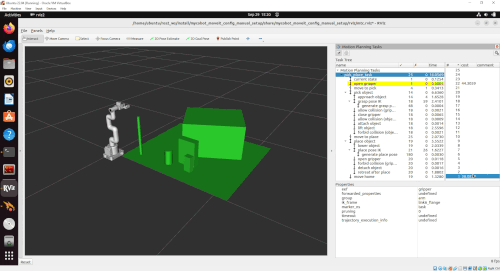
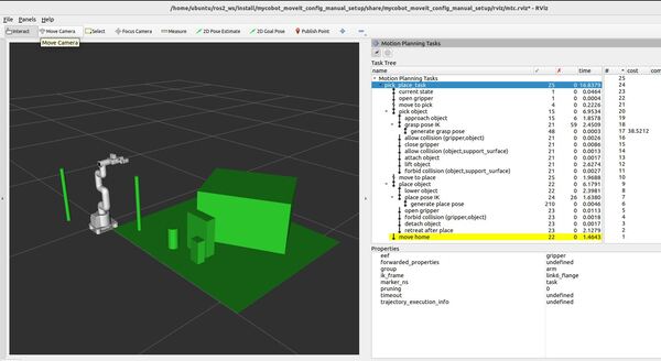
cd ~/ros2_ws/src/mycobot_ros2/hello_mtc_with_perception/src 

gedit mtc_node.cpp 

This file implements the main MoveIt Task Constructor (MTC) node for the pick and place task. It sets up the planning scene, creates the MTC task with various stages such as move to pick, grasp, lift, and place. The file also handles the execution of the task, coordinating the robot’s movements to complete the pick and place operation.

Save the file, and close it. 

gedit cluster_extraction.cpp 

This file contains functions for extracting clusters from a point cloud using a region growing algorithm. It helps in separating different objects in the scene by grouping points that likely belong to the same object. The extracted clusters can then be processed individually for object recognition or manipulation tasks.

Save the file, and close it. 

gedit get_planning_scene_client.cpp 

This file implements a test client for the GetPlanningScene service. It’s responsible for requesting the current planning scene, which includes information about objects in the environment. 

Save the file, and close it. 

gedit get_planning_scene_server.cpp 

This file implements the server for the GetPlanningScene service. It processes point cloud and RGB image data to generate CollisionObjects for the MoveIt planning scene. These CollisionObjects represent the obstacles and objects in the robot’s environment, allowing for accurate motion planning and object manipulation.

Save the file, and close it. 

gedit normals_curvature_and_rsd_estimation.cpp 

This file contains functions to estimate normal vectors, curvature values, and Radius-based Surface Descriptor (RSD) values for each point in a point cloud. These geometric features help in understanding the shape and orientation of surfaces in the scene. The estimated features can be used for tasks such as object recognition, segmentation, and grasp planning.

Save the file, and close it. 

gedit object_segmentation.cpp 

This file does most of the heavy lifting. It implements object segmentation for the input 3D point cloud. It includes functions for fitting geometric primitives (cylinders and boxes) to point cloud data, which is used to identify and represent objects in the scene.

Save the file, and close it. 

gedit plane_segmentation.cpp 

This file contains functions to segment the support plane and objects from a given point cloud. It identifies the surface on which objects are placed, separating it from the objects themselves. This segmentation is important for tasks such as determining where objects can be placed.

Save the file, and close it.

Add the Include Files

Now let’s create the header files.

cd ~/ros2_ws/src/mycobot_ros2/hello_mtc_with_perception/include 

gedit cluster_extraction.h 

Save the file, and close it.

gedit get_planning_scene_client.h 

Save the file, and close it. 

gedit normals_curvature_and_rsd_estimation.h 

Save the file, and close it. 

gedit object_segmentation.h 

Save the file, and close it. 

gedit plane_segmentation.h 

Save the file, and close it.

These header files define the interfaces for the corresponding source files we created earlier. They contain function declarations, class definitions, and necessary include statements. 

Add Launch Scripts

Let’s add some launch scripts.

cd ~/ros2_ws/src/mycobot_ros2/hello_mtc_with_perception/ 

mkdir scripts

cd scripts 

gedit pointcloud.sh 

Save the file, and close it. 

gedit robot.sh 

Save the file, and close it. 

chmod +x pointcloud.sh 

chmod +x robot.sh

These scripts will help you launch the necessary components for viewing point clouds and running the robot simulation with Gazebo, RViz, and MoveIt 2. 

The pointcloud.sh script is designed to launch the robot in Gazebo and then view a specific point cloud file. 

The robot.sh script launches the full setup including the robot in Gazebo, RViz for visualization, and sets up MoveIt 2 for motion planning. The chmod commands at the end make both scripts executable, allowing you to run them directly from the terminal.

Add the RViz Configuration File

Now let’s add the RViz configuration file.

cd ~/ros2_ws/src/mycobot_ros2/hello_mtc_with_perception/ 

mkdir rviz

cd rviz

Add the RViz configuration file.

Create a Gazebo World

cd ~/ros2_ws/src/mycobot_ros2/mycobot_gazebo/worlds/

gedit cylinder_perception.world

Save the file, and close it.

Create a Cylinder in Gazebo

Now let’s create a cylinder that we will use for pick and place in Gazebo.

cd ~/ros2_ws/src/mycobot_ros2/mycobot_gazebo/models

mkdir hello_mtc_with_perception_cylinder

cd hello_mtc_with_perception_cylinder

gedit model.sdf

Save the file, and close it.

gedit model.config

Save the file, and close it.

Create an RGBD Camera 

Let’s start by creating a URDF file for an RGBD camera. An RGBD camera captures both color (Red Green Blue) images and depth information, allowing it to see the world in 3D like human eyes do.

Gazebo has many sensors available, including one specifically for an RGBD camera.

We will add to the URDF we currently have.

cd ~/ros2_ws/src/mycobot_ros2/hello_mtc_with_perception/

mkdir urdf

cd urdf

gedit mycobot_280.urdf.xacro

Save the file, and close it.

You can see that we have put specific RGBD camera information in the <gazebo> tag so that we can specify this piece in the SDF format needed by Gazebo.

You can find many examples of SDF models here at the gz_sim Github, here are the os_gz_project_template Github, here at the ros_gz Github, and here at the gz_ros2_control Github.

mkdir meshes 

cd meshes

Add this d435.stl file.

Save the file, and close it.

Visualize the PointCloud Data in RViz

Test Point Cloud Data Generation in Gazebo

We haven’t built our package yet (using “colcon build”), but it is helpful to know how to test point cloud data in Gazebo once everything has been built. 

To confirm the point cloud data is being generated successfully in Gazebo, you would run these commands (you can come back to this section after you build the package later on in this tutorial):

ros2 launch hello_mtc_with_perception robot.launch.py use_rviz:=false

ros2 launch hello_mtc_with_perception demo.launch.py

ign topic -l (in the future, this will be “gz topic -l”)

See the information about a topic:

ign topic -t <topic_name> -i

Echo a topic:

ign topic -t <topic_name> -e

Here are some other useful commands:

ros2 launch hello_mtc_with_perception robot.launch.py use_rviz:=false

ros2 launch hello_mtc_with_perception demo.launch.py

You can run these commands to confirm data is being generated

ros2 topic echo /camera_head/depth/camera_info 

ros2 topic echo /camera_head/depth/color/points

To see the frequency of publishing, type:

ros2 topic hz /camera_head/depth/camera_info 

ros2 topic hz /camera_head/depth/color/points

To get more information on the topics, type:

ros2 topic echo /camera_head/depth/camera_info 

ros2 topic info /camera_head/color/image_raw

ros2 topic info /camera_head/depth/color/points

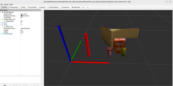
Go to RViz and click the Add button.

Click the “By topic” tab.

Click /camera_head -> /depth -> /color -> /points -> PointCloud2 so you can see the point cloud in RViz.

You can also see the camera image topic information.

Click /camera_head -> /color -> /image_raw -> Image 

Create a ROS 2 Service Interface for Point Cloud Processing for MoveIt Planning Scene Generation

Now let’s create a ROS 2 service that processes point cloud data to generate CollisionObjects for a MoveIt planning scene. This service will segment the input point cloud, fit primitive shapes to the segments, and create corresponding CollisionObjects. The service will also provide the necessary data for subsequent grasp generation should you decide to use a grasp generation strategy other than the one we will implement in this tutorial.

Here is a description of the service on a high level:

Input (Request)

• std::string: Target object shape (e.g., “cylinder”, “box”)
• std::vector<double>: Approximate target object dimensions (for identification)

Output (Response)

• moveit_msgs::msg::PlanningSceneWorld: Contains CollisionObjects for all detected objects
• sensor_msgs::msg::PointCloud2: Full scene point cloud
• sensor_msgs::msg::Image: RGB image of the scene 
• std::string: ID of the target object in the PlanningSceneWorld
• std::string: ID of the support surface in the PlanningSceneWorld
• bool: Success flag

Create a Package

Let’s create a new package called mycobot_interfaces to store our custom service definition. This package will be used across your mycobot projects for custom message and service definitions.

Here is the full package.

Navigate to your mycobot workspace:

cd ~/ros2_ws/src/mycobot_ros2

Create the new package:

ros2 pkg create --build-type ament_cmake --dependencies moveit_msgs sensor_msgs rclcpp --license BSD-3-Clause mycobot_interfaces

Navigate into the new package:

cd mycobot_interfaces

Create a srv directory for our service definitions:

mkdir srv

Update the package.xml file:

gedit package.xml

Save the file, and close it.

Update the CMakeLists.txt file:

gedit CMakeLists.txt

Save the file, and close it.

Build the package to ensure everything is set up correctly:

cd ~/ros2_ws

colcon build --packages-select mycobot_interfaces

source ~/.bashrc

Create the Custom Service Interface

Now that we have our mycobot_interfaces package set up, let’s create the custom service interface for our planning scene generation service.

Navigate to the srv directory in the mycobot_interfaces package:

cd ~/ros2_ws/src/mycobot_ros2/mycobot_interfaces/srv

Create a new file for our service definition:

gedit GetPlanningScene.srv

Add this content to define our service interface:

Save and close the file.

cd ~/ros2_ws

colcon build --packages-select mycobot_interfaces

source ~/.bashrc

Confirm Your Custom Interface

After creating our custom service interface, it’s important to verify that it has been created correctly. Follow these steps to confirm the interface creation:

Open a new terminal.

Navigate to your workspace:

cd ~/ros2_ws

Use the ros2 interface show command to display the content of our newly created service:

ros2 interface show mycobot_interfaces/srv/GetPlanningScene

Remember, whenever you make changes to your interfaces, you need to rebuild the package and source your workspace again for the changes to take effect.

Now you have created a custom service interface for planning scene generation. This service will take a target shape and dimensions as input, and return a planning scene world, full point cloud, RGB image, target object ID, support surface ID (e.g. a table), and a success flag.

To use this service in other packages, add mycobot_interfaces as a dependency in the package.xml of the hello_mtc_with_perception package where you want to use this service:

<depend>mycobot_interfaces</depend>

In your C++ code, you would include the generated header:

#include "mycobot_interfaces/srv/get_planning_scene.hpp"

You can then create service clients or servers using this interface.

This custom service interface provides a clear contract for communication between your point cloud processing node and other nodes in your system that need planning scene information.

Edit CMakeLists.txt

cd ~/ros2_ws/src/mycobot_ros2/hello_mtc_with_perception/

gedit CMakeLists.txt

Make sure your CMakeLists.txt looks like this.

Save the file, and close it.

Edit package.xml

cd ~/ros2_ws/src/mycobot_ros2/hello_mtc_with_perception/

gedit package.xml

Add this code.

Save the file, and close it.

Build the Code

cd ~/ros2_ws/

colcon build

source ~/.bashrc 

(OR source ~/ros2_ws/install/setup.bash if you haven’t set up your bashrc file to source your ROS distribution automatically with “source ~/ros2_ws/install/setup.bash”)

Launch the Code

Finally…the moment you have been waiting for.

Run the following commands (each command in a different terminal window) to launch everything:

ros2 launch hello_mtc_with_perception robot.launch.py use_rviz:=false 

ros2 launch hello_mtc_with_perception demo.launch.py 

ros2 launch hello_mtc_with_perception get_planning_scene_server.launch.py 

ros2 launch hello_mtc_with_perception run.launch.py

You can also run the robot.sh file we created earlier that does all that stuff above.

If you want to visualize the raw 3D point cloud data, you can run the pointcloud.sh script. Make sure the files are in the appropriate location.

That’s it!

Deep Learning Alternatives for MoveIt Planning Scene Generation

In the service we developed to generate the collision objects for the planning scene, we fit primitive shapes to the 3D point cloud generated by our RGBD camera. We could have also generated the MoveIt planning scene using modern deep learning methods (I won’t go through this in this tutorial).

For example, you could use a package like isaac_ros_foundationpose to create 3D bounding boxes around objects in the scene and then add those boxes as collision objects. The advantage of this technique is that you have the pose of the object as well as the class information (e.g. mug, plate, bowl, etc.)

Here is what a Detection3D.msg message would look like if you were to type ‘ros2 topic echo <name_of_detection3d_topic>’:

---
header:
  stamp:
    sec: 1694627500
    nanosec: 500000000
  frame_id: kitchen_camera
results:
  - class_id: mug
    score: 0.95
  - class_id: plate
    score: 0.03
  - class_id: bowl
    score: 0.02
bbox:
  center:
    position:
      x: 0.5
      y: 1.2
      z: 0.8
    orientation:
      x: 0.0
      y: 0.0
      z: -0.7071
      w: 0.7071
  size:
    x: 0.1
    y: 0.1
    z: 0.15
id: kitchen_mug_2

Appendix: ROS 2 Service: Generating a MoveIt Planning Scene from a 3D Point Cloud 

Overview

The method I used for generating the planning scene was inspired by the following paper: 

Goron, Lucian Cosmin, et al. “Robustly segmenting cylindrical and box-like objects in cluttered scenes using depth cameras.” ROBOTIK 2012; 7th German Conference on Robotics. VDE, 2012.

If you get a chance, I highly recommend you read this entire paper. It provides a robust methodology for generating object primitives (i.e. boxes and cylinders) from a 3D point cloud scene even if the depth camera can only see the objects partially (i.e. from one side).

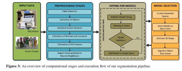
Let’s go through the technical details of the ROS 2 service we created. The purpose of the service is to process point cloud and RGB image data to generate CollisionObjects for a MoveIt planning scene. I will cover how we segmented the input point cloud, fit primitive shapes to the segments, created corresponding CollisionObjects, and provided the necessary data for subsequent grasp generation.

Service Definition

Name: get_planning_scene

Input (Request)

• std::string: Target object shape (e.g., “cylinder”, “box”)
• std::vector<double>: Approximate target object dimensions (for identification)

Output (Response)

• moveit_msgs::msg::PlanningSceneWorld: Contains CollisionObjects for all detected objects
• sensor_msgs::msg::PointCloud2: Full scene point cloud
• sensor_msgs::msg::Image: RGB image of the scene 
• std::string: ID of the target object in the PlanningSceneWorld
• std::string: ID of the support surface in the PlanningSceneWorld
• bool: Success flag

Implementation Details 

Point Cloud Preprocessing

Estimate the support plane for the objects in the scene and extract the points in the point cloud that are above the support plane (plane_segmentation.cpp)

The first step of the algorithm identifies the points that make up the flat surface (like a table) that objects are sitting on.

Input

• Point cloud (pcl::PointCloud<pcl::PointXYZRGB>)

Output

• Point cloud for the support plane
• Point cloud for the points above the detected support plane.

Process

• Estimate surface normals
  • A normal is a vector perpendicular to the surface at a given point. It provides information about the local orientation of the surface
  • For each point in the cloud, estimate the normal by fitting a plane to its k-nearest neighbors. 
  • Store the computed normals, keeping them aligned with the original point cloud. 
• Identify potential support surfaces
  • Use the computed surface normals to find approximately horizontal surfaces.
  • Group points whose normals are approximately parallel to the world Z-axis (vertical). These points likely belong to horizontal surfaces like tables.
  • Perform Euclidean clustering on these points to get support surface candidate clusters.
  • Store the support surface candidate clusters
• For each support surface candidate cluster:
  • Use RANSAC to fit a plane model
  • Validate the plane model based on the robot’s workspace limits
    • If cropping is enabled:
      • Check if the plane is within the cropped area: 
    • If cropping is disabled:
      • Skip the position check
    • Check if the plane is close to z=0:
      • Define z_tolerance (e.g., 0.05 meters)
      • Ensure the absolute value of plane_center.z is less than z_tolerance
    • Verify the plane is approximately horizontal:
      • Define up_vector as (0, 0, 1)
      • Calculate dot_product between plane_normal and up_vector
      • Define angle_tolerance based on acceptable tilt (e.g., cos of 2.5 degrees)
      • Ensure dot_product is greater than angle_tolerance
    • If all applicable conditions are met, consider the plane model valid; otherwise, reject it
• Select the best fitting plane as the support surface
  • From the set of validated plane models, choose the best candidate based on the following criteria:
    • Inlier count:
      • Define inlier_count for each plane model as the number of points that fit the model within a specified distance threshold 
      • Prefer plane models with higher inlier_count, as they represent surfaces with more supporting points
    • Plane size:
      • Calculate the area of each plane model by finding the 2D bounding box of inlier points projected onto the plane
      • Prefer larger planes, as they are more likely to represent the main support surface
    • Distance to z=0:
      • Calculate z_distance as the absolute distance of the plane’s center to z=0 
      • Prefer planes with smaller z_distance
    • Orientation accuracy:
      • Calculate orientation_score as the dot product between the plane’s normal and the up vector (0, 0, 1) 
      • Prefer planes with higher orientation_score (closer to being perfectly horizontal)
  • Combine these factors using a weighted scoring system:
    • Define weights for each factor (e.g., w_inliers, w_size, w_distance, w_orientation) 
    • Calculate a total_score for each plane model 
    • Select the plane model with the highest total_score as the best fitting plane
  • Store the selected best_plane_model for further use in object segmentation
• Return the results:
  • Create support_plane_cloud:

• Extract all inlier points from the original point cloud that belong to the best_plane_model
• Store these points in support_plane_cloud 
• Create objects_cloud:
  • For each point in the original point cloud:
    • If the point is above the best_plane_model (use the plane equation to check)
    • And if cropping is enabled, the point is within the crop boundaries
    • Add the point to objects_cloud
• Return both support_plane_cloud and objects_cloud

References:

• R. Mario and V. Markus, “Grasping of Unknown Objects from a Table Top,” in Workshop on Vision in Action: Efficient strategies for cognitive agents in complex environments, 2008.
• R. B. Rusu, N. Blodow, Z. C. Marton, and M. Beetz, “Close-range Scene Segmentation and Reconstruction of 3D Point Cloud Maps for Mobile Manipulation in Human Environments,” in IEEE/RSJ International Conference on Intelligent Robots and Systems (IROS), St. Louis, MO, USA, October 2009.

Estimate normal vectors, curvature values, and radius descriptor values for each point in the point cloud (normals_curvature_and_rsd_estimation.cpp)

Input

• Point cloud (of type pcl::PointCloudpcl::PointXYZRGB)

Output

• Point Cloud with Normal Vectors, Curvature Values, and Radius Descriptor Values
  • Each point has an associated 3D vector representing its normal vector (a 3D vector indicating the direction the surface is facing at that point)
  • Each point also has an additional value representing how curved the surface is at that point.
  • Each point has Radius-based Surface Descriptor (RSD) values (the minimum and maximum surface radius that can be fitted to the point’s neighborhood). This step determines whether a point belongs to a linear or circular surface.

Process

This approach provides a method for handling boundary points and refining normal estimation using MaximumLikelihoodSampleConsensus (MLESAC). It estimates normals, curvature, and RSD values for every point, using a more conservative approach for points identified as potentially being on a boundary.

For each point p in the cloud:

1. Find neighbors:
   • Identify the k nearest neighboring points around p (k_neighbors as input parameter)
   • These k points form the “neighborhood” of p.
   • Check if the point is a boundary point by seeing if it has fewer than k_neighbors neighbors.
   • For boundary points, adjust the neighborhood size to use a smaller number of neighbors (up to min_boundary_neighbors or whatever is available).
2. Estimate the normal vector:
   • Perform initial Principal Component Analysis (PCA) on the neighborhood:
     1. This captures how the neighborhood points are spread out around point p.
     2. The eigenvector corresponding to the smallest eigenvalue is an initial normal estimate.
   • Use Maximum Likelihood Estimation SAmple Consensus (MLESAC) to refine the local plane estimate:
     1. MLESAC aims to refine the plane fitting by robustly estimating the best plane model and discarding outliers.
     2. It uses the initial normal estimate as a starting point.
     3. If MLESAC fails, fall back to the initial normal estimate.
   • Compute a weighted covariance matrix:
     1. Assign weights to neighbor points based on their distance to the estimated local plane
     2. Points closer to the plane and inliers from MLESAC get higher weights
     3. This step helps to reduce the influence of outliers
   • Perform PCA on this weighted covariance matrix:
     1. Compute eigenvectors and eigenvalues
     2. The eigenvector corresponding to the smallest eigenvalue is the final normal estimate
3. Compute curvature values:
   • Use the eigenvalues from PCA on the weighted covariance matrix to calculate the curvature values according to the following formula: curvature = λ₀ / (λ₀ + λ₁ + λ₂) where λ₀ ≤ λ₁ ≤ λ₂
4. Calculate Radius-based Surface Descriptor (RSD) values:
   • Use pcl::RSDEstimation to compute the minimum and maximum surface radius that can be fitted to the point’s neighborhood.
   • This step determines whether a point belongs to a linear or circular surface.
5. Output creation: Point cloud that includes:
   • The original XYZ coordinates
   • The RGB color information
   • The estimated normal vector for each point
   • The estimated curvature value for each point
   • The RSD values (r_min and r_max) for each point

Key Parameters

• k_neighbors: Number of nearest neighbors to consider
• max_plane_error: Maximum allowed error for plane fitting in MLESAC
• max_iterations: Maximum number of iterations for MLESAC
• min_boundary_neighbors: Minimum number of neighbors to consider for boundary points
• rsd_radius: Radius to use for RSD estimation

References

1. R. B. Rusu, Z. C. Marton, N. Blodow, M. Dolha, and M. Beetz, “Towards 3D Point Cloud Based Object Maps for Household Environments,” Robotics and Autonomous Systems Journal (Special Issue on Semantic Knowledge in Robotics), vol. 56, no. 11, pp. 927–941, 30 November 2008.
2. Z. C. Marton, D. Pangercic, N. Blodow, and M. Beetz, “Combined 2D-3D Categorization and Classification for Multimodal Perception Systems,” International Journal of Robotics Research, 2011.

Cluster the point cloud into connected components using region growing based on nearest neighbors – cluster_extraction.cpp

Input

• Point cloud (of type pcl::PointCloud<PointXYZRGBNormalRSD>::Ptr) – Point cloud with XYZ, RGB, normal vectors, curvature values, and Radius-based Surface Descriptor (RSD) values

Output

• Vector of point cloud clusters, where each cluster is a separate point cloud containing:
  • Points that are close to each other in 3D space.
  • Each point retains its original attributes (xyz, RGB, normal, curvature, RSD values)

Process

1. Create a KdTree object for efficient nearest neighbor searches
2. Extract normals from the input cloud into a separate pcl::PointCloudpcl::Normal object
3. Create a RegionGrowing object and set its parameters:
   • Minimum and maximum cluster size
   • Number of nearest neighbors to consider
   • Smoothness threshold (angle threshold for neighboring normals)
   • Curvature threshold
4. Apply the region growing algorithm to extract clusters
5. For each extracted cluster:
   • Create a new point cloud
   • Copy points from the input cloud to the new cluster cloud based on the extracted indices
   • Set the cluster’s width, height, and is_dense properties

Key Points

• Purpose: Reduce the search space for subsequent segmentation by grouping nearby points
• Note: In cluttered scenes, objects that are touching or very close may end up in the same cluster
• This step does not perform final object segmentation, but prepares data for later segmentation steps
• The algorithm uses both geometric properties (normals) and curvature information for clustering
• Smoothness threshold is converted from degrees to radians in the implementation

Parameters

• min_cluster_size: Minimum number of points that a cluster needs to contain
• max_cluster_size: Maximum number of points that a cluster can contain
• smoothness_threshold: Maximum angle difference between normals (in degrees, converted to radians internally)
• curvature_threshold: Maximum difference in curvature between neighboring points
• nearest_neighbors: Number of nearest neighbors to consider for region growing

Additional Features

• The implementation calculates and logs various statistics for each cluster:
  • Cluster size
  • Centroid coordinates
  • Average RGB color
  • Curvature statistics (min, 20th percentile, average, median, 80th percentile, max)
  • Average RSD (Radius-based Surface Descriptor) values

References

• R. B. Rusu, N. Blodow, Z. C. Marton, and M. Beetz, “Close-range Scene Segmentation and Reconstruction of 3D Point Cloud Maps for Mobile Manipulation in Human Environments,” in IEEE/RSJ International Conference on Intelligent Robots and Systems (IROS), St. Louis, MO, USA, October 2009.

Segmentation of Clutter – object_segmentation.cpp

The input into this step is the vector of point cloud clusters that was generated during the previous step.

Input

• Vector of point cloud clusters, where each cluster is a separate point cloud containing:
  • Points that are close to each other in 3D space.
  • Each point retains its original attributes (xyz, RGB, normal, curvature, RSD values)

Output

• moveit_msgs::CollisionObject[] collision_objects

Outer Loop

The entire process below occurs for each point cloud cluster in the input vector.

Process

Project the Point Cloud Cluster Onto the Surface Plane

1. For each point (x,y,z,RGB,normal, curvature, RSDmin and RSDmax) in the 3D cluster:
   • Project the point onto the surface plane (assumed to be z=0). This creates a point (x, y).
   • Maintain a mapping between each 2D projected point and its original 3D point

Initialize Two Separate Parameter Spaces

1. Create a vector to store line models for the Hough transform
   • Each line model stores rho, theta, votes, and inlier count
2. Create a 3D Hough parameter space for circle models
   • Dimensions: center_x, center_y, radius

Understanding Hough Space

Hough space is a parameter space used for detecting specific shapes or models. Each point in Hough space represents a possible instance of the shape you’re looking for (in this case, circles or lines).

For lines:

• Instead of y = mx + b, a rho-theta parameterization of the line is used
• rho is the perpendicular distance from the line to the origin
• theta is the angle this perpendicular line makes with the X axis
• This parameterization allows for vertical lines and avoids infinite slopes

For circles:

• The Hough space is 3D: (center_x, center_y, radius)
• Each point in this space represents a possible circle in the original image

The voting process in Hough space helps find shapes even if they’re partially hidden or broken in the original image.

Inner Loop (repeated num_iterations times)

RANSAC Model Fitting

1. Line Fitting
   • Use RANSAC to fit a 2D line to the projected points. This is done to identify potential box-like objects.
2. Circle Fitting
   • Use RANSAC to fit a 2D circle to the projected points. This is done to identify cylindrical-like objects.

Filter Inliers

For the fitted models from the RANSAC Model Fitting step, apply a series of filters to refine the corresponding set of inlier points.

Circle Filtering

1. Euclidean Clustering
   • Use pcl::EuclideanClusterExtraction to group inliers into clusters.
   • Accept models with a maximum of two clusters (representing complete circles or two visible arcs of the same cylinder).
   • Reject models with more than the specified maximum number of clusters.
2. Height Consistency (for two clusters only)
   • For models with exactly two clusters, check if the height difference between clusters is within the specified tolerance.
   • This ensures that the fitted circle represents a cross-section of a single, upright cylindrical object.
3. Curvature Filtering
   • Keep inlier points with high curvature (above the specified threshold).
   • Remove inlier points with low curvature.
4. Radius-based Surface Descriptor (RSD) Filtering
   • Compare the minimum surface radius (r_min) of each inlier point to the radius of the fitted circle.
   • Keep points where the difference is within the specified tolerance.
5. Surface Normal Filtering
   • Calculate the angle between the point’s normal (projected onto the xy-plane) and the vector from the circle center to the point.
   • Keep points where this angle is within the specified threshold.

Line Filtering

1. Euclidean Clustering
   • Use pcl::EuclideanClusterExtraction to group inliers into clusters.
   • Accept models with only one cluster.
   • Reject models with more than the specified maximum number of clusters.
2. Curvature Filtering
   • Keep inlier points with low curvature (below the specified threshold).
   • Remove inlier points with high curvature.

Model Validation

For both circle and line models, check how many inlier points remain after filtering.

• If the number of remaining inliers for the model exceeds the threshold:
  • The model is considered valid.
  • Add the model to the appropriate Hough parameter space.
• If the number of remaining inliers is below the threshold:
  • The model is rejected.

An additional validation step compares inlier counts between circle and line models, keeping only the model type with more inliers.

Add Model to the Hough Space

If a model is valid:

• For circles:
  • Add a vote to the 3D Hough space (center_x, center_y, radius bins)
• For lines:
  • Add the line model (rho, theta, votes, inlier count) to the line models vector
  • rho is the perpendicular distance from the origin (0, 0) to the line
  • theta is the angle formed between the x-axis and this perpendicular vector (positive theta is counter-clockwise measured from x-axis)

Remove inliers and continue

Remove the inliers of valid models from the working point cloud and continue the inner loop until insufficient points remain or no valid models are found.

Cluster Parameter Spaces

After all iterations on a point cloud cluster:

1. Cluster line models based on similarity in rho and theta.
2. Cluster circle models in the 3D Hough space.

Select Model with Most Votes

Compare the top line cluster with the top circle cluster. Select the model type (line or circle) with the highest vote count.

Estimate 3D Shape

Using the parameters from the highest-vote cluster, fit the selected solid geometric primitive model type (box or cylinder) to the original 3D point cloud data.

Cylinder Fitting

1. Use the 2D circle fit for radius and (x,y) center position.
2. Set cylinder bottom at z=0.
3. Set top height to the highest point in the cluster.
4. Calculate dimensions and position of the cylinder.

Box Fitting

1. Compute box orientation from the line angle.
2. Project points onto the line direction and perpendicular direction to determine length and width.
3. Use z-values of points to determine height.
4. Calculate dimensions and position of the box.

Add Shape as Collision Object

The box or cylinder is added as a collision object (moveit_msgs::CollisionObject) to the planning scene with a unique id (e.g. box_0, box_1, cylinder_0, cylinder_1, etc).

Move to Next Cluster

Proceed to the next point cloud cluster in the vector (i.e., move to the next iteration of the Outer Loop).

Key Parameters

• num_iterations: Number of RANSAC iterations per cluster
• inlier_threshold: Minimum number of inliers for a model to be considered valid
• ransac_distance_threshold: Maximum distance for a point to be considered an inlier in RANSAC
• ransac_max_iterations: Maximum number of iterations for RANSAC
• circle_min_cluster_size, line_min_cluster_size: Minimum size for Euclidean clusters
• circle_max_clusters, line_max_clusters: Maximum number of allowed clusters
• circle_height_tolerance: Maximum allowed height difference between two circle clusters
• circle_curvature_threshold, line_curvature_threshold: Curvature thresholds for filtering
• circle_radius_tolerance: Tolerance for RSD filtering
• circle_normal_angle_threshold: Maximum angle between normal and radial vector for circles
• circle_cluster_tolerance, line_cluster_tolerance: Distance threshold for Euclidean clustering
• line_rho_threshold, line_theta_threshold: Thresholds for clustering line models in the parameter space

Get Planning Scene Server (get_planning_scene_server.cpp)

This code brings together all the previously developed components into a single, unified ROS 2 service. It integrates functions for point cloud processing, plane segmentation, object clustering, and shape fitting into a cohesive workflow. The service processes point cloud and RGB image data to generate a MoveIt planning scene, which can be called by a node using the MoveIt Task Constructor to obtain environment information for manipulation tasks. The core functionality is encapsulated in the handleService method of the GetPlanningSceneServer class.

handleService Method Walkthrough

1. Initialize Response: The method starts by setting the success flag of the response to false.
2. Check Data Availability: It verifies that both point cloud and RGB image data are available. If either is missing, it logs an error and returns.
3. Validate Input Parameters and Prepare Point Cloud:
   • Checks if target_shape and target_dimensions are valid
   • Transforms the point cloud to the target frame
   • Applies optional cropping to the point cloud
4. Convert PointCloud2 to PCL Point Cloud: Converts the ROS PointCloud2 message to a PCL point cloud for further processing.
5. Segment Support Plane and Objects: Uses the segmentPlaneAndObjects function to separate the support surface from objects in the scene.
6. Create CollisionObject for Support Surface: Generates a CollisionObject representing the support surface and adds it to the planning scene.
7. Estimate Normals, Curvature, and RSD: Calls estimateNormalsCurvatureAndRSD to calculate geometric features for each point in the object cloud.
8. Extract Clusters: Uses extractClusters to identify distinct object clusters in the point cloud.
9. Get Collision Objects: Calls segmentObjects to convert point cloud clusters into collision objects for the planning scene.
10. Identify Target Object: Searches through the collision objects to find one matching the requested target shape and dimensions.
11. Assemble PlanningSceneWorld: Combines all collision objects into a complete PlanningSceneWorld structure.
12. Fill the Response:
    • Sets the full point cloud, RGB image, target object ID, and support surface ID in the response
    • Sets the success flag to true if all critical steps were successful
    • Logs detailed information about the response contents

This method transforms raw sensor data into a structured planning scene that can be used by the MoveIt Task Constructor for motion planning and manipulation tasks.

Congratulations on reaching the end! Keep building!